What do you think?
Rate this book

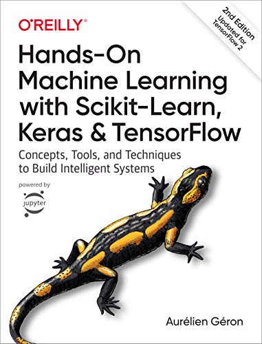
Through a series of recent breakthroughs, deep learning has boosted the entire field of machine learning. Now, even programmers who know close to nothing about this technology can use simple, efficient tools to implement programs capable of learning from data. This practical book shows you how.
By using concrete examples, minimal theory, and two production-ready Python frameworks—Scikit-Learn and TensorFlow—author Aurélien Géron helps you gain an intuitive understanding of the concepts and tools for building intelligent systems. You’ll learn a range of techniques, starting with simple linear regression and progressing to deep neural networks. With exercises in each chapter to help you apply what you’ve learned, all you need is programming experience to get started.
Explore the machine learning landscape, particularly neural nets Use Scikit-Learn to track an example machine-learning project end-to-end Explore several training models, including support vector machines, decision trees, random forests, and ensemble methods Use the TensorFlow library to build and train neural nets Dive into neural net architectures, including convolutional nets, recurrent nets, and deep reinforcement learning Learn techniques for training and scaling deep neural nets851 pages, ebook
First published April 9, 2017