Philip Nelson's Blog

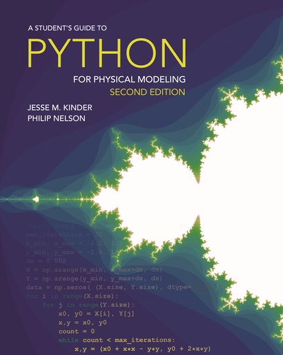
We are pleased to announce the second edition of A Student’s Guide to Python for Physical Modeling!

The book will be available in early August, in time for fall classes.

We have updated the book to reflect changes in the language, and we have added new material on methods that have become more prominent in scientific programming in recent years — such as data science and version control. The second edition is about 70 pages longer than the updated edition. However, we maintained the concise, hands-on approach of earlier editions and worked diligently to make the text clear and easy to follow.

New Material

Our first task was to bring everything up to date so that readers can build a working Python environment from scratch. Everything from installation instructions to screenshots have been brought up to date.

We also developed and tested all code with the latest version of Python: Python 3.9. We made a deliberate effort to use simple constructs and standard libraries, so the code samples run with earlier versions of Python, too.

(The “latest version” of an open-source software package is a quickly moving target. With Python’s new release schedule, any version number in print is guaranteed to be out of date in less than a year! If you want to explore the latest changes to the Python language, you can read about what’s new..)

The bulk of the new material in the second edition comes in two new chapters.

Chapter 10 — Advanced Techniques introduces several Python programming tools that are advanced for someone new to computer programming, but are also indispensable to scientific computing:

Dictionaries and generatorsTools for data science and machine learning: pandas and scikit-learn (a very brief introduction)Symbolic computing with SymPy (greatly expanded coverage from earlier editions, with a guided investigation of the first passage problem)Python classes (a tutorial in writing classes to study random walks in 1, 2, or 3 dimensions and on a variety of lattices)

Appendix B — Command Line Tools introduces readers to working at the command line: a UNIX/Linux shell, a macOS terminal, or the Anaconda Prompt in Windows. It also introduces Git for version control. (You can now obtain the entire repository of code samples from GitHub!)

Introduction to navigating the file system from the command lineCreating, moving, and deleting files and directoriesUsing a text editor from the command lineVersion control with Git

There are many other updates and additions throughout the rest of the text, too.

Raw strings (convenient for LaTeX)Comparison of plt.subplot and plt.subplotsHeat maps with pcolormeshComplex root finding with fsolveSolving ODE’s with solve_ivp

We have also added several new code samples and “Your Turn” exercises — with solutions — so readers can try out the new techniques.

Thanks to the many readers who provided helpful comments and suggestions on earlier editions of the book. We look forward to your feedback on the second edition!

This blog accompanies A Student’s Guide to Python for Physical Modeling by Jesse M. Kinder and Philip Nelson.

A Student’s Guide provides an introduction to the Python computer language and a few libraries (NumPy, SciPy, and PyPlot) that will enable students to get started in physical modeling. Some of the topics covered include the following:

basic Python programmingimporting and exporting datanumerical arrays2D and 3D plottingMonte Carlo simulationsnumerical integrationsolving ordinary differential equationssymbolic mathematicsanimationimage processing

You can have a look at the Table of Contents.

On this Web site, you will find data sets, code samples, errata, addtional resources, and extended discussions of the topics introduced in the book.

Enjoy!

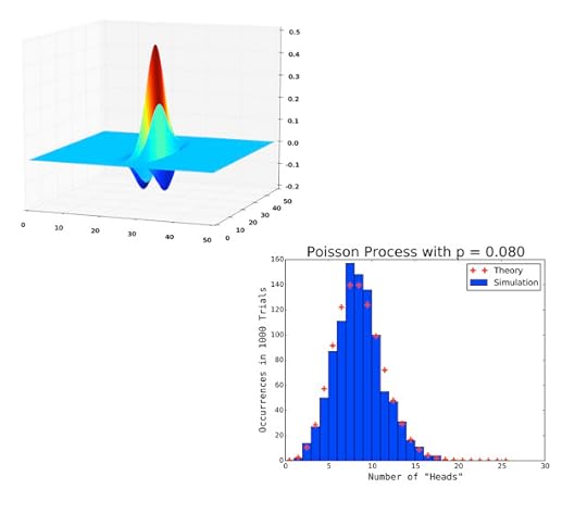Plots created with NumPy and PyPlot.

Happy New Year!

We are pleased to start off 2018 by announcing that the updated edition of A Student's Guide to Python for Physical Modeling is now available!

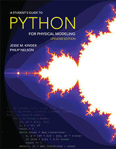
The hard copy edition is shipping and is available from Princeton University Press. You can expedite your order by calling the distributor directly at (800) 343-4499. (The ISBN is 9780691180571.) The Kindle edition is currently available for pre-order on Amazon. The book will be available from other distributors, along with e-book editions, in the near future.

This blog accompanies A Student’s Guide to Python for Physical Modeling by Jesse M. Kinder and Philip Nelson.

A Student’s Guide provides an introduction to the Python computer language and a few libraries (NumPy, SciPy, and PyPlot) that will enable students to get started in physical modeling. Some of the topics covered include the following:

basic Python programmingimporting and exporting datanumerical arrays2D and 3D plottingMonte Carlo simulationsnumerical integrationsolving ordinary differential equationssymbolic mathematicsanimationimage processing

You can have a look at the Table of Contents.

On this Web site, you will find data sets, code samples, errata, addtional resources, and extended discussions of the topics introduced in the book.

Enjoy!

Plots created with NumPy and PyPlot.

We have been busy working on A Student’s Guide to Python for Physical Modeling this summer. We are preparing an updated edition for Winter of 2018. We wanted to take this opportunity to alert readers to a few items that have changed since the publication of the first edition, back in 2015.

Python 3.6

The “latest version” of any software package is a moving target, and putting a version number in print ensures that it will be outdated at some point in the future. In the first edition, we used Python 3.4. The latest stable release of Python is version 3.6, and Python 3.7 is under development. Happily, all of the code samples in the book run with Python 3.6.

One change that came with Python 3.5 may be of interest to scientific programmers. Python introduced a new operator for matrix multiplication: the “@” symbol. NumPy recognizes this operator, and it can be used as shorthand for the np.dot() function. This may allow you to write simpler, more intuitive code, which usually leads to fewer errors.

x = np.random.random(3)
M = np.random.random((3,3))

x @ M == np.dot(x,M)
M @ x == np.dot(M,x)

If you want to explore the latest changes to Python, you can read about what’s new.

Goodbye, Continuum. Hello, Anaconda, Inc.

Continuum Analytics is no more. The company has changed its name to Anaconda, Inc. One significant result of this decision is that many of the Web links in the first edition — Appendix A (Installation) in particular — may no longer work in the future.

The new home page of Anaconda is now anaconda.com. This is where you can download the Anaconda distribution of Python and find all of the official Anaconda documentation. The old continuum.io links in the first edition will probably continue to work for some time, but if you find a broken link, you may need to search for the relevant material at anaconda.com instead.

The Anaconda distribution has evolved over time. Some of the instructions in Appendix A of the first edition for command line installation with the condapackage manager are now unnecessary:

The Anaconda distribution now includes the mkl package by default.

The accelerate package has evolved into something beyond the scope of our book. You can read about it here.

Installing spyder with Miniconda is now even simpler. As of August 2017, we found no missing packages when installing spyder with the condapackage manager. There is no need to install jinja2, docutils, or pyflakes separately.

Errata

Since publication of A Student’s Guide to Python for Physical Modeling, we have discovered a few errors. We have recently updated the Errata on this Web site. Happily, the list is short. All of these will be corrected in the upcoming revised edition. Thanks to all of the alert readers who brought these to our attention!

Updated Edition

Some readers may be wondering what will be changed in the updated edition. We did not feel the changes were substantial enough to justify calling the work a “second edition,” but we did put a lot of work into improving the text:

We corrected all known errors.

We made many changes merely to bring the content of the book up to date with the constantly changing content of the World Wide Web and open-source software packages.

We added an introduction to Jupyter notebooks. Our blog post provided an outline for the new material.

We added a discussion of 2D histograms.

We added a discussion of displaying data as images with plt.imshow.

Much of our effort went into reorganizing and rewriting the original material so that that it will be clearer and easier to follow. We hope that anyone who reads the two editions side by side will find much that is improved, even if there is not a lot that is new.

Suppose you have written a Python script that carries out a simulation based on a physical model and creates a nice plot of the results. Now you wish to explore the model and run the calculation on many different sets of input parameters. What is the best way to proceed?

You could write a script that runs the same calculation on a list of inputs that you select ahead of time:

inputs = [(x0, y0, z0), (x1, y1, z1), (x2, y2, z2)]
for I in inputs:
# Insert simulation code here.

You could place your script inside a function and call the function repeatedly from the IPython command line with different inputs:

def run_simulation(x, y, z):
# Insert simulation code here.

Both methods work, but both neither is ideal. If you use a script with an input list, you have to select the inputs ahead of time. If you find an interesting region of parameter space, you have to modify the script and run it again. If you embed your simulation within a function, you have to do a lot of typing at the command line.

A simple graphical user interface (GUI) that runs the script would be a convenient way to explore the model. You could enter your inputs in the appropriate boxes — or even set them with slider bars — and run the simulation; change one, and run it again. Such an interface would also make it much easier for someone else to run your code.

This post will describe how to create a simple graphical user interface (GUI) for your own functions and scripts using the Tkinter module. The goal is not to provide an introduction to GUI development or to create a beautiful user interface. Instead, this post will focus on building a minimal GUI wrapper for a working Python program. You can learn how to add the bells and whistles later.

Anatomy of a GUI

Take a look at the screenshot of the GUI below. This post will describe how to construct it from scratch.

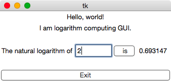A simple GUI.

A GUI is an interactive window that controls a program or series of programs. It allows the user to provide input to and receive feedback from those programs. Before getting into the details of creating this particular GUI, let’s examine a few of the key ideas behind GUI programming.

A GUI is built from widgets.

A widget is, in essence, anything you can put inside a GUI. These are the fundamental units from which a GUI is built:

Text Boxes: These are inactive widgets that simply display a text message.

Entry Boxes: These are interactive text boxes. The user can enter text or numbers. The data in an entry box can be extracted and used within programs.

Buttons: These are interactive regions of the GUI. When the user clicks on a button, it usually causes something to happen. The button can display explanatory text.

Widgets are packed into frames.

A frame is an abstract region of the GUI occupied by a widget or collection of widgets. The GUI program will arrange frames within the GUI window and try to adjust the size of the frames to fill the available space.

We will pack widgets into frames by creating a widget, then specifying which frame to put it in. We can provide additional information about where it is to be placed, like “top”, “bottom”, “left”, or “right”.

We can also pack frames within frames. For instance, in the GUI above, the third line of the window contains a text box, an entry box, a button, and another text box that displays the result of the calculation. All of these widgets were packed into a single frame, then this frame was packed within the application window frame.

Events trigger actions.

When we interact with a GUI, we expect something to happen. An event is something that happens within the GUI: you press a key or click on a button. GUI programming links events like these to specific actions. The great thing about building your own GUIs is that you get to choose both the events and the actions.

A program runs when you click on a <Run> button.

A variable is updated when you click the mouse in a certain region of the window.

A calculation is carried out after you press <Enter> in a text box.

The window closes when you press the <Escape> key.

Events are bound to widgets.

When creating a GUI, we bind events to specific widgets. For instance, if you create a <Press Here> button, you get to assign the event “click mouse on <Press Here> button” to anything you like:

do nothingdisplay a messagemake noiseevaluate a numerical calculationrun a Monte Carlo simulationcreate a plotexit the program

The same event can have different effects with different widgets: pressing <Escape> in an entry box may clear the entry, but pressing <Escape> outside of the entry box may close the window.

A Word on GUI Design

It is easy to get distracted by all of the options available in GUI programming, by all of the features you could add, by all of the fine-tuning you can do to the appearance and interface. To avoid getting sidetracked, you should plan before you write any code:

Decide which events are necessary. If your goal is to enter the value of two parameters, then run a simulation, stick to that. Anything else is unnecessary.

Decide which widgets you need to carry out your task. For the example above, we might use two entry boxes and a <Run> button. Perhaps some explanatory text boxes would also be helpful. The 3D control knobs for adjusting parameter values can wait …

Make a quick sketch of the layout. This will help you in packing your minimal set of widgets into the window.

Now you are ready to build a GUI!

The Tkinter Module

To actually construct a GUI, we need to choose a GUI programming library. Tkinter is the standard GUI library for Python, and it is included with almost every Python distribution. It has the benefits of being widely available and platform-independent. (I.e., you can create a GUI for Windows, Mac OS X, or Linux with the same Python code.) There are many other options, but this post will focus exclusively on Tkinter.

Tkinter provides an object-oriented framework for GUI programming. There are objects like Frame, Label, Entry, and Button that implement the widgets we need. We will build a GUI by creating a collection of these objects, then using their methods to adjust their properties and pack them together into a single window.

To gain access to the Tkinter module, we must import it. In my scripts I use the following lines:

try:
# This will work in Python 2.7
import Tkinter
except ImportError:
# This will work in Python 3.5
import tkinter as Tkinter

For some reason, Python 3 uses the lower-case tkinter while Python 2.7 uses the upper-case Tkinter. The lines above will work with either environment and allow us to access the module as Tkinter.

There is one more caveat for those who use the Anaconda distribution of Python. If you are going to use PyPlot and Tkinter in the same program, you need to instruct PyPlot to use a Tk-based back end for displaying plots:

import matplotlib
matplotlib.use('TkAgg')
import matplotlib.pyplot as plt

If you do not set the back end before importing PyPlot, you may see a bunch of error messages instead of your GUI, even if you never call a PyPlot command.

Some Simple GUIs

The first few GUIs we build will be simple and not very useful, but they will illustrate the basic properties of any GUI.

Your First GUI

Together with the import lines above, the following two lines will create the simplest GUI possible: an empty window that does absolutely nothing.

# Create main window.
root = Tkinter.Tk()

# Activate the window.
root.mainloop()

The first command creates an object for the window that will contain the entire GUI. According to the docstrings of Tkinter.Tk, this object is a

Toplevel widget of Tk which represents mostly the main window
of an application. It has an associated Tcl interpreter.

This command should probably come near the top of your program. Later, we will pack all of our widgets and frames into this master widget.

The second command should come near the end of your program. It launches the window. Any code you type after this command will not have any effect until the window closes.

Try the import command and the two commands above to make sure you can create a Tkinter window on your system. You should see a blank application window with the title “tk”. The window you create may not appear in the foreground. You can close it by clicking on the close button, as you would any other application.

Adding a Widget

Now let’s add the simplest possible widget to our GUI — a text box — and pack it into the main window.

# Create main window.
root = Tkinter.Tk()

# Create a text box and pack it in.
greeting = Tkinter.Label(text="Hello, world!")
greeting.pack()

# Activate the window.
root.mainloop()

Note how the widget was created. I created a variable greeting and assigned it to a Tkinter.Label object. When I created the object, I used the keyword argument text="Hello, world!" to set the message. Then, I packed this newly created widget into the main window.

If you run this script, you will see the effect of packing a single widget. The resulting window is tiny — just large enough to contain the text message. The widgets are packed into the smallest amount of space that will contain them.

Binding an Event to a Keystroke

Next, we will bind an event to a keystroke within the main window. With the following script, you can now close the window by pressing the <Escape> key as long as the window is active.

# Create main window.
root = Tkinter.Tk()

# Create a text box and pack it in.
greeting = Tkinter.Label(text="Hello, world!")
greeting.pack()

# Define a function to close the window.
def quit(event=None):
root.destroy()

# Cause pressing <Esc> to close the window.
root.bind('<Escape>', quit)

# Activate the window.
root.mainloop()

Notice the procedure used here. First, I defined a function that carried out some action. In this case, it calls the destroy() method of the rootwindow, closing the window. Next, I used the bind() method of the root window to associate this function with a particular event: “user presses the <Escape>key.” Note that you pass only the function name to the bind() method — no arguments and no parentheses. The following would have produced an error:

root.bind('<Escape>', quit() )

Some Tkinter methods pass an event object to the function they are given, and some do not. To accommodate both types of methods, I gave my function an optional argument with a default value.

If you want to bind an event to a mouse click instead of a keystroke, use '<Button-1>' as the “key”. Add the following lines to the script above, just before the root.mainloop() command:

def ring(event=None):
root.bell()

root.bind('<Button-1>', ring)

Now you will here a beep any time you click the mouse inside the main window.

Binding an Event to a Widget

You can also bind events to specific widgets within the main window. Let’s add a button to close the window.

# Create main window.
root = Tkinter.Tk()

# Create a text box and pack it in.
greeting = Tkinter.Label(text="Hello, world!")
greeting.pack()

# Define a function to close the window.
def quit(event=None):
root.destroy()

# Cause pressing <Esc> to close the window.
root.bind('<Escape>', quit)

# Create a button that will close the window.
button = Tkinter.Button(text="Exit", command=quit)
button.pack(side='bottom', fill='both')

# Activate the window.
root.mainloop()

In this example, I have created a button with some text and bound it to the quit() command that closes the window. Notice, also, that I have provided instructions for where the button is to be placed: side='bottom'. I also specified that the button should be expanded to fill all of the available space around it in the frame.

Entry Boxes, Variables, and Frames

Now, let’s look at the last few elements we will need to create a useful GUI.

An entry box allows you to pass information to programs called by the GUI. In order for the GUI to keep track of the variables it contains, we need to assign the data in an entry box to a Tkinter variable. Tkinter recognizes several types: IntVar for integers, DoubleVar for floats, StringVar for strings. I prefer to use strings to store exactly what the user types, then convert this to other types as needed.

If you provide an entry box, it is often useful to provide a text box that indicates what the user is entering. This can create a problem in packing: You want the text box and entry box to be side by side, but the program that arranges all of our widgets in the main window might not arrange things in an aesthetically pleasing manner. The solution is to pack the text box and entry box into a separate frame, then pack this frame into the application window.

The script logarithm.py below illustrates all of these ideas. Liberal comments explain all of the steps in the construction of this GUI, which computes the logarithm of a number entered by the user. You can evaluate the logarithm by pressing the “is” button or by pressing <Enter> in the entry box.

A Useful GUI

Now it is time to assemble everything into a useful application. The script ‘interference.py’ below creates a GUI wrapper that allows the user to set the amplitude and frequency of two waves. The function it calls adds the two waves together and displays the resulting interference pattern.

It uses one new construct: a grid for arranging the input text boxes and entry boxes. Instead of calling widget.pack() to place a widget, one calls widget.grid(I, J) to place the widget in cell (I,J) of a grid. The upper left corner of the grid is cell (0,0).

This script is not a sterling example of GUI programming. The functions that do the numerical calculation and create the graph should defined in a separate module so that they can be run with or without the GUI. The GUI wrapper should import the function that creates the plot from this module. However, ‘interference.py’ has the benefit of being self-contained: you can copy and paste it into your own editor and run it without further modification.

Once you understand the basics of constructing a GUI wrapper for a program, you can simplify the process by writing functions to help create the GUI! For instance, you could write a function that takes a list of variable names and automatically generates a grid of text and entry boxes.

And there are always embellishments. You could replace entry boxes with sliders for some variables. (Look up Tkinter.Scale.) You can add check boxes for Boolean variables. (Look up Tkinter.Checkbutton.) You can add menus and save dialogs and … well, you get the picture. Just don’t spend so much time building a fancy interface that you have none left to actually run the simulation!

Summary

This post covered a lot of ground quickly, but I hope it has provided enough information for you to create a GUI window to run your own scripts whenever this is a useful thing to do. (Many programs do not benefit from a GUI at all, and it is not useful to create a GUI for a program that does not yet run properly …)

Design a GUI before you start building it. Decide what it should do first. Then identify the widgets that will accomplish your goal and sketch the layout of the application before you write any GUI code. The Tkinter module available with most Python distributions provides a suite of tools for building GUIs in Python.

This post has only scratched the surface of the Tkinter module and has completely ignored other GUI programming libraries. A Web search for “Tkinter” or “GUI programming with Python” will reveal a wealth of resources for more advanced GUI programming.

Code Samples The logarithm.py Module # -----------------------------------------------------------------------------
# logarithm.py
# -----------------------------------------------------------------------------
"""
Create a GUI application to compute logarithms using the Tkinter module.
"""
try:
# This will work in Python 2.7
import Tkinter
except ImportError:
# This will work in Python 3.5
import tkinter as Tkinter

# -----------------------------------------------------------------------------
# Create main window.
# -----------------------------------------------------------------------------
root = Tkinter.Tk()

# Create two text boxes and pack them in.
greeting = Tkinter.Label(text="Hello, world!")
greeting.pack(side='top')

advertisement = Tkinter.Label(text="I am logarithm computing GUI.")
advertisement.pack(side='top')

# Define a function to close the window.
def quit(event=None):
root.destroy()

# Cause pressing <Esc> to close the window.
root.bind('<Escape>', quit)

# Create a button that will close the window.
button = Tkinter.Button(text="Exit", command=quit)
button.pack(side='bottom', fill='both')

# -----------------------------------------------------------------------------
# Create a frame within the main window.
# -----------------------------------------------------------------------------
# The frame will contain the widgets needed to do a calculation.
# Each widget in "frame" is created with "frame" as its first argument.
frame = Tkinter.Frame(root)
frame.pack(side='top')

# Create a text box that explains the calculation.
invitation = Tkinter.Label(frame, text="The natural logarithm of")
invitation.pack(side='left')

# Define an input variable and add an entry box so the user can change its value.
x = Tkinter.StringVar()
x.set('2.71828')
x_entry = Tkinter.Entry(frame, width=8, textvariable=x)
x_entry.pack(side='left')

# Define an output variable and a function to compute its value.
y = Tkinter.StringVar()

def compute_y(event=None):
from math import log
# Get x and y from outside the function.
global x, y

# Get the string value of the x StringVar and convert it to a float.
x_value = float(x.get())

# Compute the floating point value of y.
y_value = log(x_value)

# Convert this to a formatted string, and store it in the y StringVar.
y.set('%.6f' % y_value)

# Bind an event to the x_entry box: pressing <Enter> will calculate the
# logarithm of whatever number the user has typed.
x_entry.bind('<Return>', compute_y)

# Create a button to perform the calculation and pack it into the frame.
compute = Tkinter.Button(frame, text=' is ', command=compute_y)
compute.pack(side='left')

# Create a text box that displays the value of the y StringVar.
y_label = Tkinter.Label(frame, textvariable=y, width=8)
y_label.pack(side='left')

# -----------------------------------------------------------------------------
# Activate the window.
# -----------------------------------------------------------------------------
root.mainloop()
The interference.py Module # -----------------------------------------------------------------------------
# interference.py
# -----------------------------------------------------------------------------
"""
Author: Jesse M. Kinder
Created: 2016 Apr 15
Modified: 2016 Apr 15

Description
-----------
Build a GUI wrapper to explore the interference pattern of two waves.
"""
try:
# This will work in Python 2.7
import Tkinter
except ImportError:
# This will work in Python 3.5
import tkinter as Tkinter

# -----------------------------------------------------------------------------
# To use matplotlib, the author must use the TkAgg backend, or none of this will
# work and a long string of inexplicable error messages will ensue.
# -----------------------------------------------------------------------------
import matplotlib
matplotlib.use('TkAgg')
import numpy as np
import matplotlib.pyplot as plt

# Define a bold font:
BOLD = ('Courier', '24', 'bold')

# Create main application window.
root = Tkinter.Tk()

# Create a text box explaining the application.
greeting = Tkinter.Label(text="Create an Interference Pattern", font=BOLD)
greeting.pack(side='top')

# Create a frame for variable names and entry boxes for their values.
frame = Tkinter.Frame(root)
frame.pack(side='top')

# Variables for the calculation, and default values.
amplitudeA = Tkinter.StringVar()
amplitudeA.set('1.0')
frequencyA = Tkinter.StringVar()
frequencyA.set('1.0')

amplitudeB = Tkinter.StringVar()
amplitudeB.set('1.0')
frequencyB = Tkinter.StringVar()
frequencyB.set('1.0')

deltaPhi = Tkinter.StringVar()
deltaPhi.set('0.0')

# Create text boxes and entry boxes for the variables.
# Use grid geometry manager instead of packing the entries in.
row_counter = 0
aa_text = Tkinter.Label(frame, text='Amplitude of 1st wave:')
aa_text.grid(row=row_counter, column=0)

aa_entry = Tkinter.Entry(frame, width=8, textvariable=amplitudeA)
aa_entry.grid(row=row_counter, column=1)

row_counter = 1
fa_text = Tkinter.Label(frame, text='Frequency of 1st wave:')
fa_text.grid(row=row_counter, column=0)

fa_entry = Tkinter.Entry(frame, width=8, textvariable=frequencyA)
fa_entry.grid(row=row_counter, column=1)

row_counter = 1
ab_text = Tkinter.Label(frame, text='Amplitude of 2nd wave:')
ab_text.grid(row=row_counter, column=0)

ab_entry = Tkinter.Entry(frame, width=8, textvariable=amplitudeB)
ab_entry.grid(row=row_counter, column=1)

row_counter = 1
fb_text = Tkinter.Label(frame, text='Frequency of 2nd wave:')
fb_text.grid(row=row_counter, column=0)

fb_entry = Tkinter.Entry(frame, width=8, textvariable=frequencyB)
fb_entry.grid(row=row_counter, column=1)

row_counter = 1
dp_text = Tkinter.Label(frame, text='Phase Difference:')
dp_text.grid(row=row_counter, column=0)

dp_entry = Tkinter.Entry(frame, width=8, textvariable=deltaPhi)
dp_entry.grid(row=row_counter, column=1)

# Define a function to create the desired plot.
def make_plot(event=None):
# Get these variables from outside the function, and update them.
global amplitudeA, frequencyA, amplitudeB, frequencyB, deltaPhi

# Convert StringVar data to numerical data.
aa = float(amplitudeA.get())
fa = float(frequencyA.get())
ab = float(amplitudeB.get())
fb = float(frequencyB.get())
phi = float(deltaPhi.get())

# Define the range of the plot.
t_min = -10
t_max = 10
dt = 0.01
t = np.arange(t_min, t_max dt, dt)

# Create the two waves and find the combined intensity.
waveA = aa * np.cos(fa * t)
waveB = ab * np.cos(fb * t phi)
intensity = (waveA waveB)**2

# Create the plot.
plt.figure()
plt.plot(t, intensity, lw=3)
plt.title('Interference Pattern')
plt.xlabel('Time')
plt.ylabel('Intensity')
plt.show()


# Add a button to create the plot.
MakePlot = Tkinter.Button(root, command=make_plot, text="Create Plot")
MakePlot.pack(side='bottom', fill='both')

# Allow pressing <Return> to create plot.
root.bind('<Return>', make_plot)

# Allow pressing <Esc> to close the window.
root.bind('<Escape>', root.destroy)

# Activate the window.
root.mainloop()

Happy New Year!

Let’s start off 2016 by learning something new: Jupyter Notebooks, formerly known as IPython Notebooks.

A Jupyter notebook is an interactive document that incorporates text, math, graphics, and code. It can be viewed in a Web browser. Unlike most documents, however, you can modify and execute the code inside the document. In this sense, a Jupyter notebook is similar to a session in Mathematica or Maple. The difference is that the interpreter running behind the scenes is not Mathematica or Maple. Jupyter notebooks were designed to run Julia, Python, and R, but they support over 40 languages at present.

The best way to learn about Jupyter notebooks is to take a look at one. This notebook is a simple example from a greenhorn, but you can find many more on the Web.

Introduction.ipynb

Click on the link to view the notebook. You can download the notebook using the Save icon at the upper right corner of the notebook Web page. You can then open the notebook, run it, and see the commands used to create it.

In my very limited experience, I find that notebooks are excellent for sharingcode but not for developing code. An IDE like Spyder or working from the command line is more efficient for writing and debugging code, running scripts repeatedly, and generating complex graphics. However, once the scripts and modules are working properly, you can call them within a notebook.

Jupyter notebooks are great for exploring new ideas and solving problems. A Jupyter notebook allows you to integrate formatted text, mathematical formulas, Python code, and graphics into a single document. You can write about your ideas, do mathematical analyses, write and run code, view graphics, and reflect on the results without switching applications.

Even if you do not like to do all of your work on your laptop or in the computer lab — I still prefer pencil and paper for many tasks — Jupyter notebooks are a great option for writing up your work and sharing it with others. A Jupyter notebook is like a word processor that can also run Python code. You can keep detailed notes with working code for your own personal files. You can write up homework assignments. You can write reports to share your work with other scientists. You can publish your work on the Web. (The procedure for sharing a notebook over the Internet can be found here.) A notebook can be exported in several formats, including HTML. If you have LaTeX installed on your system, you can also convert the notebook to a PDF file.

If you would like to see more examples of notebooks, explore this gallery. Enjoy!

How do you get your Python interpreter to find modules that are not located in your current working directory? The answer is … you tell it where to look.

When you type something like

from my_module import my_function

Python searches a collection of directories (i.e., folders) on your computer. If the directory containing <my_module.py> is not in this collection, you will receive an ImportError. This can be frustrating if you know the file exists, and even more so if you know where it exists.

In this post, we will take a brief look at how to add paths to the collection of directories searched by Python.

Paths

A path is essentially a set of directions to a file:

/Users/username/modules/my_module.py [Mac OS X, Linux]
C:\modules\my_module.py [Windows]

It tells your operating system how to navigate from a fixed starting point — the “root directory” / in Unix-based systems, or C:\ in Windows — through a collection of folders to the desired file.

In this case, there is a folder called <modules/> that contains the desired file, <my_module.py>. Let’s suppose that you are writing a script called <my_script.py> in your working directory:

/Users/username/scratch/my_script.py [Mac OS X, Linux]
C:\scratch\my_script.py [Windows]

You want Python to import <my_module.py> when you run the script, but it cannot find the file.

Below are 4 options for adding the path for your module to Python’s collection of paths. None are extremely complicated, but the last two require working with the command line and editing startup files on your operating system. If you are unfamiliar or uncomfortable with this, you might prefer the first two methods.

You will need to replace directory names like /Users/username/ or C:\scratch\ with the correct directories on your own system for these examples to work.

Using The sys Module

There is a module called sys that lets you modify the collection of paths from within Python. According to its documentation,

This module provides access to some objects used or maintained by the
interpreter and to functions that interact strongly with the interpreter.

One of these objects is a list called sys.path. Again referring to the documentation,

path -- module search path

All we need to do is add the path to <my_module.py> to sys.path. On Unix-like systems, the commands are

import sys
sys.path.append('/Users/username/modules')

On Windows, it is easier to use a raw string to specify the path:

import sys
sys.path.append(r'c:\modules')

This will only affect the path in the current Python session. If you quit and restart, you will need to add the path again.

Using Spyder

If you are using the Spyder IDE, you can permanently add a directory to its collection of paths. Chose the “PYTHONPATH manager” from the menu (python > PYTHONPATH manager) as shown below:

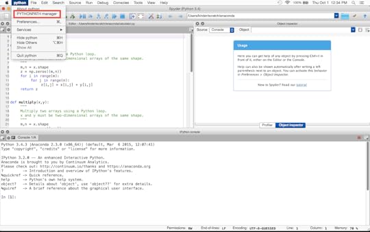Managing paths within Spyder.

This will open a window that shows a list of directories added to Spyder’s collection of paths. If you have not modified this list already, it will probably contain your working directory and nothing else. At the bottom of this window, there is an icon for “Add Path”. Click on this. Now you can find the directory you want to add, as if you were opening a file.

In this case, we navigate to

/Users/username/modules

and select “Choose”.

Once you have selected a directory, it will become a permanent addition to Python’s paths within Spyder. You will need to quit Spyder and restart or “Restart Kernel” for the changes to take effect.

This is a convenient way to access modules that are not part of the Anaconda distribution from within Spyder.

Using the Command Line

If you are working from a command line, you can add your module directory to Python’s collection of paths by setting the PYTHONPATH variable before you start a Python session or run a script:

$ export PYTHONPATH=${PYTHONPATH}:/Users/username/modules
$ python my_script.py

No matter what directory you are working in, Python now knows where to find <my_module.py>.

If you want to permanently add your module directory to PYTHONPATH, you can add the export command above to your <.profile> or <.bashrc> file.

Startup Files

Another option is to create a Python startup file — a Python script that will be run at the beginning of every interactive Python session (but not when you run scripts from the command line). First, create a file such as <python_startup.py> in your home directory. Then, enter Python commands exactly as you would type them at the command prompt:

# python_startup.py
# Startup script for interactive Python sessions.

import sys
sys.path.append('/Users/username/modules')

Next, edit your <.profile> or <.bashrc> file and add the line

export PYTHONSTARTUP=/Users/username/python_startup.py

And that’s it. Now, every time you start a new Python session, you can access your own modules.

IPython does not use the PYTHONSTARTUP variable. If you want to add a startup script for IPython, place a file like <python_startup.py> in IPython’s directory of startup scripts:

/Users/username/.ipython/default_profile/startup/

Now your modules will be available in every IPython session, including Spyder.

Summary

There are several ways to show Python where to find modules. For a single session, appending a path to the sys.path variable is an easy solution. For a permanent change, you can use Spyder’s PYTHONPATH manager or edit startup files from the command line. These methods will allow you to access modules without copying or moving files into your working directory, and you can easily access modules you write yourself or modules you download from the Web.

The goal of this post and its predecessor is to provide some toolsand tips for improving the performance of Python programs. In the previouspost, we examined profiling tools — sophisticated stopwatchesfor timing programs as they execute. In this post, we will use these tools todemonstrate some general principles that make Python programs run faster.

Remember: If your program already runs fast enough, you do not need to worryabout profiling and optimization. Faster is not always better, especially ifyou end up with code that is difficult to read, modify, or maintain.

Overview

We can summarize our principles for optimizing performance as follows:

Debug first. Never attempt to optimize a program that does not work.Focus on bottlenecks. Find out what takes the most time, and work onthat.Look for algorithmic improvements. A different theoretical approachmight speed up your program by orders of magnitude.Use library functions. The routines in NumPy, SciPy, and PyPlot havealready been optimized.Eliminate Python overhead. Iterating over an index takes more time thanyou think.

If fast code is important to you, you can start writing new code with theseguidelines in mind and apply them to existing code to improve performance.

Debug first.

Your primary objective in programming is to produce a working program. Unlessthe program already does what it is supposed to do, there is no point in tryingto speed it up. Profiling and optimization are not part of debugging. Theycome afterward.

Focus on bottlenecks.

The greatest gains in performance come from improving the most time-consumingportions of your program. The profiling tools described in Part 1of this two-part post can help you identify bottlenecks — portions of aprogram that limit its overall performance. They can also help you identifyfaster alternatives. Once you have identified the bottlenecks in your program,apply the other principles of optimization to mitigate or eliminate them.

Look for algorithmic improvements.

The greatest gains in speed often come from using a different algorithm to solveyour problem.

When comparing algorithms, one analyzes how the computation time scales withsome measure of the size of the problem. Some number \(N\) usually characterizesthe size of a problem — e.g., the number of elements in a vector or the number ofitems in a list. The time required for a program to run is expressed as afunction of \(N\). If an algorithm scales as \(N^3\), it means that when \(N\) islarge enough, doubling \(N\) will cause the algorithm to take roughly 8 times aslong to run. If you can find an algorithm with better scaling, you can oftenimprove the performance of your program by orders of magnitude.

As an example, consider the classic problem of sorting a jumbled list ofnumbers. You might consider using the following approach:

Create an empty list to store the sorted numbers.Find the smallest item in the jumbled list.Remove the smallest item from the jumbled list and place it at the end of thesorted list.Repeat steps 2 and 3 until there are no more items in the jumbled list.

This method is calledinsertion sort.It works, and it is fast enough for sorting small lists. You can prove thatsorting a jumbled list of \(N\) elements using an insertion sort will require onthe order of \(N^2\) operations. That means that sorting a list with 1 millionentries will take 1 million times longer than sorting a list of 1000 entries.That may take too long, no matter how much you optimize!

Delving into a computer science textbook, you might discover mergesort, a different algorithm thatrequires on the order of \(N \log N\) operations to sort a jumbled list of \(N\)elements. That means that sorting a list of 1 million entries will take roughly6000 times longer than sorting a list of 1000 entries — not 1 million. Forbig lists, this algorithm is orders of magnitude faster, no matter whatprogramming language you are using.

As another example, you might need to determine a vector \(\mathbf{x}\) in thelinear algebra problem \(A \cdot \mathbf{x} = \mathbf{b}\). If \(A\) is an \(N\times N\) matrix, then inverting \(A\) and multiplying the inverse with\(\mathbf{b}\) takes on the order of \(N^3\) operations. You quickly reach thelimits of what your computer can handle around \(N = 10,000\). However, if yourmatrix has some special structure, there may be an algorithm that takes advantageof that structure and solve the problem much faster. For example, if \(A\) issparse (most of its elements are zero), you can reduce the scaling to \(N^2\) —or even \(N\) — instead of \(N^3\). That is a huge speedup if \(N = 10,000\)!These kinds of algorithmic improvements make an “impossible” calculation“trivial”.

Unfortunately, there is no algorithm for discovering better algorithms. It isan active branch of computer science. You need to understand your problem,delve into texts and journal articles, talk to people who do research in thefield, and think really hard. The payoff is worth the effort.

Use library functions.

Once you have a working program and you have identified the bottlenecks, you areready to start optimizing your code. If you are already using the bestavailable algorithms, the simplest way to improve the performance of Python codein most scientific applications is to replace homemade Python functions withlibrary functions.

It’s not that you are a bad coder! It’s just that someone else took the time torewrite a time-consuming operation in C or FORTRAN, compile and optimize it,then provide you with a simple Python function to access it. You are simplytaking advantage of work that someone else has already done.

Let’s use the profiling tool %timeit to look at a some examples of the speeduppossible with library functions.

Building an array of random numbers

Suppose you need an array of random numbers for a simulation. Here is aperfectly acceptable function for generating the array:

import numpy as npdef Random(N): """ Return an array of N random numbers in the range [0,1). """ result = np.zeros(N) for i in range(N): result[i] = np.random.random() return result

This code works and it is easy to understand, but suppose my program does notrun fast enough. I need to increase the size of the simulation by a factor of10, but it already takes a while. After debugging and profiling, I see thatthe line of my program that calls Random(N) takes 99 percent the executiontime. That is a bottleneck worth optimizing!

I can start by profiling this function:

$ %timeit Random(1000)1000 loops, best of 3: 465 us per loop

When I look at the documentation for np.random.random, I discover it iscapable of doing more than generate a single random number. Maybe I should justuse it to generate the entire array …

$ %timeit np.random.random(1000)10000 loops, best of 3: 28.9 us per loop

I can generate exactly the same array in just 6 percent of the time!

In this hypothetical example, my entire program will run almost 20 times faster.I can increase the size of my calculation by a factor of 10 and reduce theoverall calculation time simply by replacing Random(N) by np.random.random(N).

Array operations

Let’s look at an even more dramatic example. In the previous post,I introduced a library to add, multiply, and take the square root of arrays.(The library, calculator.py is included at the bottom of thispost.) Suppose, once again, I have identified the bottleneck in aworking program, and it involves the functions in the calculator.py module.

NumPy has equivalent operations with the same names. (When you write x y fortwo arrays, it is shorthand for np.add(x,y).) Let’s see how much we can speedthe operations up by switching to the NumPy equivalents. First, import themodules and create two random two-dimensional arrays to act on:

import calculator as calcimport numpy as npx = np.random.random((100,100))y = np.random.random((100,100))

Now, time the operations in calculator.py and NumPy:

$ %timeit calc.add(x,y)100 loops, best of 3: 9.76 ms per loop$ %timeit np.add(x,y)100000 loops, best of 3: 18.8 us per loop

Here we see an even more significant difference. The addition function writtenin pure Python takes 500 times longer to add the two arrays. Use %timeit tocompare calc.multiply with np.multiply, and calc.sqrt with np.sqrt, andyou will see similar results.

When to write your own functions

The implications of these examples are clear: NumPy array operations are much,much faster than the equivalent Python code. The same is true of specialfunctions in the SciPy and PyPlot packages and many other Python libraries. Tospeed up your code, use functions from existing libraries when possible. Thiscan save time in writing code, optimizing code, and running code.

So should you ever write your own functions?

I was once told, “Never write your own linear algebra routines. Somebodyalready wrote a faster one in the 1970s.” That may be generally true, but it isbad advice nonetheless. If you never write your own routine to invert a matrix,it is difficult to fully understand how these routines work and when they canfail, and you will certainly never discover a better algorithm.

If speed of execution is not important or if your goal is to understand how analgorithm works, you should write your own functions. If you need to speed up aworking Python program, look to library functions.

Eliminate Python overhead.

Why are library functions are so much faster than their Python equivalents? Theanswer is a point we discussed in Chapter 2 of A Student’s Guide to Python forPhysical Modeling: In Python, everything is an object. When you type“x = 1”, Python does not just store the value 1 in a memory cell. Itcreates an object endowed with many attributes and methods, one of which is thevalue 1. Type dir(1) to see all of the attributes and methods of aninteger.

What’s more, Python has no way of knowing what type of objects are involved in asimple statement like z = x y. First, it has to determine what kind of objectx is and what kind of object y is (type-checking). Then it has tofigure out how to interpret “ ” for these two objects. If the operation makessense, Python then has to create a new object to store the result of x y.Finally, it has to assign this new object to the name z. This gives Python alot of flexibility: x and y can be integers, floats, arrays, lists, strings,or just about anything else. This flexibility makes it easy to write programs,but it also adds to the total computation time.

To speed up programs, eliminate this overhead. In other words, make Pythondo as little as possible.

Using library functions from NumPy, SciPy, and PyPlot eliminates overhead, andthis is the main reason they run so much faster. In the example above,np.add(x,y) is not doing anything fundamentally different thancalc.add(x,y); it simply does addition and iteration in the background,without Python objects. Recall from the previous post thatcalc.add(x,y) spent almost 30 percent of its time iterating of the index jin the inner for loop.

Other ways to eliminate overhead are

Use in-place operations. Operations like =, -=, *=, and /=operate on an existing object instead of creating a new one.Use built-in methods. These methods are often optimized.Use list comprehensions and generators instead of forloops. Initializing a list and accessing its elements take time.Vectorize your code. (Section 2.5.1 of A Student’s Guide to Python forPhysical Modeling )

Use %timeit to compare the performance of these functions. They use theprinciples above to eliminate some of the Python overhead in square_list0.

def square_list0(N): """ Return a list of squares from 0 to N-1. """ squares = [] for n in range(N): squares = squares [n**2] return squaresdef square_list1(N): """ Return a list of squares from 0 to N-1. """ squares = [] for n in range(N): # In-place operations: Replace "x = x ..." with "x = ..." squares = [n**2] return squares def square_list2(N): """ Return a list of squares from 0 to N-1. """ squares = [] for n in range(N): # Built-in methods: Replace "x = x ..." with "x.append(...)" squares.append(n**2) return squares def square_list3(N): """ Return a list of squares from 0 to N-1. """ # Use list comprehension instead of for loop. return [n**2 for n in range(N)] def square_array(N): """ Return an array of squares from 0 to N-1. """ # Vectorize the entire operation. from numpy import arange return arange(N)**2

In my tests, square_list3(1000) ran about 18 times faster thansquare_list0(1000), and square_array(N) was about 350 times faster thansquare_list0(1000). The last function virtually eliminates Python overheadby using NumPy arrays in vectorized code.

More Options

If performance is still not satisfactory after attempting the optimizationsdescribed here, you can try compiling your Python code. Compiling is beyond thescope of this post. You can find out more aboutNumba(which is included in the Anaconda distribution) orCythonby following these links. Numba allows you to compile pure Python code. Cythonallows you to write fast C extensions for Python without learning C.

For users of the Anaconda distribution of Python, there is an optional add-oncalled Accelerate. This add-onwill replace the standard NumPy, SciPy, and other scientific libraries withequivalent libraries that use Intel’s MKL routines for linear algebra. On manymachines, this will improve performance without any effort on your part beyondinstalling the package. Accelerate also includes NumbaPro, a proprietaryversion of the Numba package. Accelerate is free to academic users.

Summary

To summarize, there are a few simple ways to speed up a Python program. Onceyou have a working program and you have identified its bottlenecks, you can lookfor library functions to replace the slowest functions in your program, you canrewrite your code to eliminate Python’s overhead, and you can search for fasteralgorithms to solve your problem. As you develop your programming skills, youwill start to incorporate these principles automatically. Happily, this meansless time profiling and optimizing!

Code SamplesThe calculator.py Module# -----------------------------------------------------------------------------# calculator.py# ----------------------------------------------------------------------------- """This module uses NumPy arrays for storage, but executes array math using Pythonloops."""import numpy as npdef add(x,y): """ Add two arrays using a Python loop. x and y must be two-dimensional arrays of the same shape. """ m,n = x.shape z = np.zeros((m,n)) for i in range(m): for j in range(n): z[i,j] = x[i,j] y[i,j] return zdef multiply(x,y): """ Multiply two arrays using a Python loop. x and y must be two-dimensional arrays of the same shape. """ m,n = x.shape z = np.zeros((m,n)) for i in range(m): for j in range(n): z[i,j] = x[i,j] * y[i,j] return zdef sqrt(x): """ Take the square root of the elements of an arrays using a Python loop. """ from math import sqrt m,n = x.shape z = np.zeros((m,n)) for i in range(m): for j in range(n): z[i,j] = sqrt(x[i,j]) return zdef hypotenuse(x,y): """ Return sqrt(x**2 y**2) for two arrays, a and b. x and y must be two-dimensional arrays of the same shape. """ xx = multiply(x,x) yy = multiply(y,y) zz = add(xx, yy) return sqrt(zz)

The goal of this post and its predecessor is to provide some tools and tips for improving the performance of Python programs. In the previous post, we examined profiling tools — sophisticated stopwatches for timing programs as they execute. In this post, we will use these tools to demonstrate some general principles that make Python programs run faster.

Remember: If your program already runs fast enough, you do not need to worry about profiling and optimization. Faster is not always better, especially if you end up with code that is difficult to read, modify, or maintain.

Overview

We can summarize our principles for optimizing performance as follows:

Debug first. Never attempt to optimize a program that does not work.Focus on bottlenecks. Find out what takes the most time, and work on that.Look for algorithmic improvements. A different theoretical approach might speed up your program by orders of magnitude.Use library functions. The routines in NumPy, SciPy, and PyPlot have already been optimized.Eliminate Python overhead. Iterating over an index takes more time than you think.

If fast code is important to you, you can start writing new code with these guidelines in mind and apply them to existing code to improve performance.

Debug first.

Your primary objective in programming is to produce a working program. Unless the program already does what it is supposed to do, there is no point in trying to speed it up. Profiling and optimization are not part of debugging. They come afterward.

Focus on bottlenecks.

The greatest gains in performance come from improving the most time-consuming portions of your program. The profiling tools described in Part 1of this two-part post can help you identify bottlenecks — portions of a program that limit its overall performance. They can also help you identify faster alternatives. Once you have identified the bottlenecks in your program, apply the other principles of optimization to mitigate or eliminate them.

Look for algorithmic improvements.

The greatest gains in speed often come from using a different algorithm to solve your problem.

When comparing algorithms, one analyzes how the computation time scales with some measure of the size of the problem. Some number \(N\) usually characterizes the size of a problem — e.g., the number of elements in a vector or the number of items in a list. The time required for a program to run is expressed as a function of \(N\). If an algorithm scales as \(N^3\), it means that when \(N\) is large enough, doubling \(N\) will cause the algorithm to take roughly 8 times as long to run. If you can find an algorithm with better scaling, you can often improve the performance of your program by orders of magnitude.

As an example, consider the classic problem of sorting a jumbled list of numbers. You might consider using the following approach:

Create an empty list to store the sorted numbers.Find the smallest item in the jumbled list.Remove the smallest item from the jumbled list and place it at the end of the sorted list.Repeat steps 2 and 3 until there are no more items in the jumbled list.

This method is called insertion sort. It works, and it is fast enough for sorting small lists. You can prove that sorting a jumbled list of \(N\) elements using an insertion sort will require on the order of \(N^2\) operations. That means that sorting a list with 1 million entries will take 1 million times longer than sorting a list of 1000 entries. That may take too long, no matter how much you optimize!

Delving into a computer science textbook, you might discover merge sort, a different algorithm that requires on the order of \(N \log N\) operations to sort a jumbled list of \(N\)elements. That means that sorting a list of 1 million entries will take roughly 6000 times longer than sorting a list of 1000 entries — not 1 million. For big lists, this algorithm is orders of magnitude faster, no matter what programming language you are using.

As another example, you might need to determine a vector \(\mathbf{x}\) in the linear algebra problem \(A \cdot \mathbf{x} = \mathbf{b}\). If \(A\) is an \(N \times N\) matrix, then inverting \(A\) and multiplying the inverse with \(\mathbf{b}\) takes on the order of \(N^3\) operations. You quickly reach the limits of what your computer can handle around \(N = 10,000\). However, if your matrix has some special structure, there may be an algorithm that takes advantage of that structure and solve the problem much faster. For example, if \(A\) is sparse (most of its elements are zero), you can reduce the scaling to \(N^2\) — or even \(N\) — instead of \(N^3\). That is a huge speedup if \(N = 10,000\)! These kinds of algorithmic improvements make an “impossible” calculation “trivial”.

Unfortunately, there is no algorithm for discovering better algorithms. It is an active branch of computer science. You need to understand your problem, delve into texts and journal articles, talk to people who do research in the field, and think really hard. The payoff is worth the effort.

Use library functions.

Once you have a working program and you have identified the bottlenecks, you are ready to start optimizing your code. If you are already using the best available algorithms, the simplest way to improve the performance of Python code in most scientific applications is to replace homemade Python functions with library functions.

It’s not that you are a bad coder! It’s just that someone else took the time to rewrite a time-consuming operation in C or FORTRAN, compile and optimize it, then provide you with a simple Python function to access it. You are simply taking advantage of work that someone else has already done.

Let’s use the profiling tool %timeit to look at a some examples of the speedup possible with library functions.

Building an array of random numbers

Suppose you need an array of random numbers for a simulation. Here is a perfectly acceptable function for generating the array:

import numpy as np

def Random(N):
"""
Return an array of N random numbers in the range [0,1).
"""
result = np.zeros(N)
for i in range(N):
result[i] = np.random.random()
return result

This code works and it is easy to understand, but suppose my program does not run fast enough. I need to increase the size of the simulation by a factor of 10, but it already takes a while. After debugging and profiling, I see that the line of my program that calls Random(N) takes 99 percent the execution time. That is a bottleneck worth optimizing!

I can start by profiling this function:

$ %timeit Random(1000)
1000 loops, best of 3: 465 us per loop

When I look at the documentation for np.random.random, I discover it is capable of doing more than generate a single random number. Maybe I should just use it to generate the entire array …

$ %timeit np.random.random(1000)
10000 loops, best of 3: 28.9 us per loop

I can generate exactly the same array in just 6 percent of the time!

In this hypothetical example, my entire program will run almost 20 times faster. I can increase the size of my calculation by a factor of 10 and reduce the overall calculation time simply by replacing Random(N) by np.random.random(N).

Array operations

Let’s look at an even more dramatic example. In the previous post, I introduced a library to add, multiply, and take the square root of arrays. (The library, calculator.py is included at the bottom of this post.) Suppose, once again, I have identified the bottleneck in a working program, and it involves the functions in the calculator.py module.

NumPy has equivalent operations with the same names. (When you write x y for two arrays, it is shorthand for np.add(x,y).) Let’s see how much we can speed the operations up by switching to the NumPy equivalents. First, import the modules and create two random two-dimensional arrays to act on:

import calculator as calc
import numpy as np
x = np.random.random((100,100))
y = np.random.random((100,100))

Now, time the operations in calculator.py and NumPy:

$ %timeit calc.add(x,y)
100 loops, best of 3: 9.76 ms per loop

$ %timeit np.add(x,y)
100000 loops, best of 3: 18.8 us per loop

Here we see an even more significant difference. The addition function written in pure Python takes 500 times longer to add the two arrays. Use %timeit to compare calc.multiply with np.multiply, and calc.sqrt with np.sqrt, and you will see similar results.

When to write your own functions

The implications of these examples are clear: NumPy array operations are much, much faster than the equivalent Python code. The same is true of special functions in the SciPy and PyPlot packages and many other Python libraries. To speed up your code, use functions from existing libraries when possible. This can save time in writing code, optimizing code, and running code.

So should you ever write your own functions?

I was once told, “Never write your own linear algebra routines. Somebody already wrote a faster one in the 1970s.” That may be generally true, but it is bad advice nonetheless. If you never write your own routine to invert a matrix, it is difficult to fully understand how these routines work and when they can fail, and you will certainly never discover a better algorithm.

If speed of execution is not important or if your goal is to understand how an algorithm works, you should write your own functions. If you need to speed up a working Python program, look to library functions.

Eliminate Python overhead.

Why are library functions are so much faster than their Python equivalents? The answer is a point we discussed in Chapter 2 of A Student’s Guide to Python for Physical Modeling: In Python, everything is an object. When you type “x = 1”, Python does not just store the value 1 in a memory cell. It creates an object endowed with many attributes and methods, one of which is the value 1. Type dir(1) to see all of the attributes and methods of an integer.

What’s more, Python has no way of knowing what type of objects are involved in a simple statement like z = x y. First, it has to determine what kind of object x is and what kind of object y is (type-checking). Then it has to figure out how to interpret “ ” for these two objects. If the operation makes sense, Python then has to create a new object to store the result of x y. Finally, it has to assign this new object to the name z. This gives Python a lot of flexibility: x and y can be integers, floats, arrays, lists, strings, or just about anything else. This flexibility makes it easy to write programs, but it also adds to the total computation time.

To speed up programs, eliminate this overhead. In other words, make Python do as little as possible.

Using library functions from NumPy, SciPy, and PyPlot eliminates overhead, and this is the main reason they run so much faster. In the example above, np.add(x,y) is not doing anything fundamentally different than calc.add(x,y); it simply does addition and iteration in the background, without Python objects. Recall from the previous post that calc.add(x,y) spent almost 30 percent of its time iterating of the index jin the inner for loop.

Other ways to eliminate overhead are

Use in-place operations. Operations like =, -=, *=, and /=operate on an existing object instead of creating a new one.Use built-in methods. These methods are often optimized.Use list comprehensions and generators instead of for loops. Initializing a list and accessing its elements take time.Vectorize your code. (Section 2.5.1 of A Student’s Guide to Python for Physical Modeling )

Use %timeit to compare the performance of these functions. They use the principles above to eliminate some of the Python overhead in square_list0.

def square_list0(N):
"""
Return a list of squares from 0 to N-1.
"""
squares = []
for n in range(N):
squares = squares [n**2]
return squares


def square_list1(N):
"""
Return a list of squares from 0 to N-1.
"""
squares = []
for n in range(N):
# In-place operations: Replace "x = x ..." with "x = ..."
squares = [n**2]
return squares


def square_list2(N):
"""
Return a list of squares from 0 to N-1.
"""
squares = []
for n in range(N):
# Built-in methods: Replace "x = x ..." with "x.append(...)"
squares.append(n**2)
return squares


def square_list3(N):
"""
Return a list of squares from 0 to N-1.
"""
# Use list comprehension instead of for loop.
return [n**2 for n in range(N)]


def square_array(N):
"""
Return an array of squares from 0 to N-1.
"""
# Vectorize the entire operation.
from numpy import arange
return arange(N)**2

In my tests, square_list3(1000) ran about 18 times faster than square_list0(1000), and square_array(N) was about 350 times faster than square_list0(1000). The last function virtually eliminates Python overhead by using NumPy arrays in vectorized code.

More Options

If performance is still not satisfactory after attempting the optimizations described here, you can try compiling your Python code. Compiling is beyond the scope of this post. You can find out more about Numba(which is included in the Anaconda distribution) or Cythonby following these links. Numba allows you to compile pure Python code. Cython allows you to write fast C extensions for Python without learning C.

For users of the Anaconda distribution of Python, there is an optional add-on called Accelerate. This add-on will replace the standard NumPy, SciPy, and other scientific libraries with equivalent libraries that use Intel’s MKL routines for linear algebra. On many machines, this will improve performance without any effort on your part beyond installing the package. Accelerate also includes NumbaPro, a proprietary version of the Numba package. Accelerate is free to academic users.

Summary

To summarize, there are a few simple ways to speed up a Python program. Once you have a working program and you have identified its bottlenecks, you can look for library functions to replace the slowest functions in your program, you can rewrite your code to eliminate Python’s overhead, and you can search for faster algorithms to solve your problem. As you develop your programming skills, you will start to incorporate these principles automatically. Happily, this means less time profiling and optimizing!

Code Samples The calculator.py Module # -----------------------------------------------------------------------------
# calculator.py
# -----------------------------------------------------------------------------
"""
This module uses NumPy arrays for storage, but executes array math using Python
loops.
"""

import numpy as np

def add(x,y):
"""
Add two arrays using a Python loop.
x and y must be two-dimensional arrays of the same shape.
"""
m,n = x.shape
z = np.zeros((m,n))
for i in range(m):
for j in range(n):
z[i,j] = x[i,j] y[i,j]
return z


def multiply(x,y):
"""
Multiply two arrays using a Python loop.
x and y must be two-dimensional arrays of the same shape.
"""
m,n = x.shape
z = np.zeros((m,n))
for i in range(m):
for j in range(n):
z[i,j] = x[i,j] * y[i,j]
return z


def sqrt(x):
"""
Take the square root of the elements of an arrays using a Python loop.
"""
from math import sqrt
m,n = x.shape
z = np.zeros((m,n))
for i in range(m):
for j in range(n):
z[i,j] = sqrt(x[i,j])
return z


def hypotenuse(x,y):
"""
Return sqrt(x**2 y**2) for two arrays, a and b.
x and y must be two-dimensional arrays of the same shape.
"""
xx = multiply(x,x)
yy = multiply(y,y)
zz = add(xx, yy)
return sqrt(zz)