
Terence Tao's Blog
November 24, 2025
Call for industry sponsors for IPAM’s RIPS program
Over the last 25 years, the Institute for pure and applied mathematics (IPAM) at UCLA (where I am now director of special projects) has run the popular Research in Industrial Projects for Students (RIPS) program every summer, in which industry sponsors with research projects are matched with talented undergraduates and a postdoctoral mentor to work at IPAM on the sponsored project for nine weeks. IPAM is now putting out a call for industry sponsors who can contribute a suitable research project for the Summer of 2026, as well as funding to cover the costs of the research; details are available here.
(Student applications for this program will open at a later date, once the list of projects is finalized.)


November 21, 2025
Climbing the cosmic distance ladder: another sample chapter
Five years ago, I announced a popular science book project with Tanya Klowden on the cosmic distance ladder, in which we released a sample draft chapter of the book, covering the “fourth rung” of the ladder, which for us meant the distances to the planets. In the intervening time, a number of unexpected events have slowed down this project significantly; but I am happy to announce that we have completed a second draft chapter, this time on the “seventh rung” of measuring distances across the Milky Way, which required the maturation of the technologies of photography and spectroscopy, as well as the dawn of the era of “big data” in the early twentieth century, as exemplified for instance by the “Harvard computers“.
We welcome feedback of course, and are continuing to work to complete the book despite the various delays. In the mean time, you can check out our instagram account for the project, or the pair of videos that Grant Sanderson (3blue1brown) produced with us on this topic, which I previously blogged about here.
Thanks to Clio Cresswell and Noah Klowden for comments and corrections.
November 19, 2025
Sum-difference exponents for boundedly many slopes, and rational complexity
I have uploaded to the arXiv my paper “Sum-difference exponents for boundedly many slopes, and rational complexity“. This is the second spinoff of my previous project with Bogdan Georgiev, Javier Gómez–Serrano, and Adam Zsolt Wagner that I recently posted about. One of the many problems we experimented using the AlphaEvolve tool with was that of computing sum-difference constants. While AlphaEvolve did modest improve one of the known lower bounds on sum-difference constants, it also revealed an asymptotic behavior to these constants that had not been previously observed, which I then gave a rigorous demonstration of in this paper.
In the original formulation of the sum-difference problem, one is given a finite subset  of
of  with some control on projections, such as

 and
and  for every
  , one gets a family of line segments whose set of directions has cardinality (1), but whose slices at heights
  have cardinality at most
  .
.Because  is clearly determined by
  and
and  , one can trivially get an upper bound of
  on (1). In 1999, Bourgain utilized what was then the very recent “Balog–Szemerédi–Gowers lemma” to improve this bound to
  , which gave a new lower bound of
  on the (Minkowski) dimension of Kakeya sets in
  , which improved upon the previous bounds of Tom Wolff in high dimensions. (A side note: Bourgain challenged Tom to also obtain a result of this form, but when they compared notes, Tom obtained the slightly weaker bound of
  , which gave Jean great satisfaction.) Currently, the best upper bound known for this quantity is
  .
.
One can get better bounds by adding more projections. For instance, if one also assumes

 . The arithmetic Kakeya conjecture asserts that, by adding enough projections, one can get the exponent arbitrarily close to
  . If one could achieve this, this would imply the Kakeya conjecture in all dimensions. Unfortunately, even with arbitrarily many projections, the best exponent we can reach asymptotically is
  .
.It was observed by Ruzsa that all of these questions can be equivalently formulated in terms of Shannon entropy. For instance, the upper bound of (1) turns out to be equivalent to the entropy inequality

 (not necessarily independent) taking values in . In the language of this paper, we write this as
As part of the AlphaEvolve experiments, we directed this tool to obtain lower bounds for 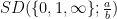 for various rational numbers
  , defined as the best constant in the inequality

 as
as  :
:
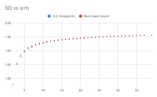
The first main result of this paper is to confirm that this is indeed the case, in that

 is in lowest terms and not equal to
  , where
  are absolute constants. The lower bound was obtained by observing the shape of the examples produced by AlphaEvolve, which resembled a discrete Gaussian on a certain lattice determined by
  . The upper bound was established by an application of the “entropic Plünnecke–Ruzsa calculus”, relying particularly on the entropic Ruzsa triangle inequality, the entropic Balog–Szemerédi–Gowers lemma, as well as an entropy form of an inequality of Bukh.
The arguments also apply to settings where there are more projections under control than just the  projections. If one also controls projections
  for various rationals
  and
and  denotes the set of slopes of the projections under control, then it turns out that the associated sum-difference constant
  still decays to , but now the key parameter is not the height
  of
of  , but rather what I call the rational complexity of with respect to , defined as the smallest integer
  for which one can write as a ratio
  where
where  are integer-coefficient polynomials of degree at most and coefficients at most
  . Specifically, decays to at a polynomial rate in , although I was not able to pin down the exponent of this decay exactly. The concept of rational complexity may seem somewhat artificial, but it roughly speaking measures how difficult it is to use the entropic Plünnecke–Ruzsa calculus to pass from control of
  , and
, and  to control of
  .
.
While this work does not make noticeable advances towards the arithmetic Kakeya conjecture (we only consider regimes where the sum-difference constant is close to , rather than close to ), it does highlight the fact that these constants are extremely arithmetic in nature, in that the influence of projections  on is highly dependent on how efficiently one can represent as a rational combination of the
  .
.
November 12, 2025
New Nikodym set constructions over finite fields
I have uploaded to the arXiv my paper “New Nikodym set constructions over finite fields“. This is a spinoff of my previous project with Bogdan Georgiev, Javier Gómez–Serrano, and Adam Zsolt Wagner that I recently posted about. In that project we experimented with using AlphaEvolve (and other tools, such as DeepThink and AlphaProof) to explore various mathematical problems which were connected somehow to an optimization problem. For one of these — the finite field Nikodym set problem — these experiments led (by a somewhat convoluted process) to an improved asymptotic construction of such sets, the details of which are written up (by myself rather than by AI tools) in this paper.
Let  be a finite field of some order
  (which must be a prime or a power of a prime), and let
  be a fixed dimension. A Nikodym set in
  is a subset of with the property that for every point
  , there exists a line
  passing through
  such that all points of other than lie in . Such sets are close cousins of Kakeya sets (which contain a line in every direction); indeed, roughly speaking, applying a random projective transformation to a Nikodym set will yield (most of) a Kakeya set. As a consequence, any lower bound on Kakeya sets implies a similar bound on Nikodym sets; in particular, one has a lower bound
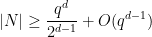
, coming from a similar bound on Kakeya sets due to Bukh and Chao using the polynomial method.For Kakeya sets, Bukh and Chao showed this bound to be sharp up to the lower order error  ; but for Nikodym sets it is conjectured that in fact such sets should asymptotically have full density, in the sense that
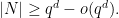
) by Guo, Kopparty, and Sudan by combining the polynomial method with the theory of linear codes. But in other cases this conjecture remains open in three and higher dimensions.In our experiments we focused on the opposite problem of constructing Nikodym sets of size as small as possible. In the plane  , constructions of size when is a perfect square were constructed by Blokhuis et al, again using the theory of blocking sets; by taking Cartesian products of such sets, one can also make similar constructions in higher dimensions, again assuming is a perfect square. Apart from this, though, there are few such constructions in the literature.
We set AlphaEvolve to try to optimize the three dimensional problem with a variable field size (which we took to be prime for simplicity), with the intent to get this tool to come up with a construction that worked asymptotically for large , rather than just for any fixed value of . After some rounds of evolution, it arrived at a construction which empirically had size about  . Inspecting the code, it turned out that AlphaEvolve had constructed a Nikodym set by (mostly) removing eight low-degree algebraic surfaces (all of the form
  for various
  ). We used the tool DeepThink to confirm the Nikodym property and to verify the construction, and then asked it to generalize the method. By removing many more than eight surfaces, and using some heuristic arguments based on the Chebotarev density theorem, DeepThink claimed a construction of size formed by removing several higher degree surfaces, but it acknowledged that the arguments were non-rigorous.
The arguments can be sketched here as follows. Let  be a random surface of degree , and let be a point in
  which does not lie in . A random line through then meets in a number of points, which is basically the set of zeroes in of a random polynomial of degree . The (function field analogue of the) Chebotarev density theorem predicts that the probability that this polynomial has no roots in is about
  , where
elements that are derangements (no fixed points). So, if one removes  random surfaces of degrees
  , the probability that a random line avoids all of these surfaces is about
  . If this product is significantly greater than
  , then the law of large numbers (and concentration of measure) then predicts (with high probability) that out of the
  lines through , at least one will avoid the removed surfaces, thus giving (most of) a Nikodym set. The Lang-Weil estimate predicts that each surface has cardinality about
  , so this should give a Nikodym set of size about
  .
.DeepThink took the degrees to be large, so that the derangement probabilities  were close to
  . This led it to predict that could be taken to be as large as
  , leading to the claimed bound (2). However, on inspecting this argument we realized that these moderately high degree surfaces were effectively acting as random sets, so one could dramatically simplify DeepThink’s argument by simply taking to be a completely random set of the desired cardinality (2), in which case the verification of the Nikodym set property (with positive probability) could be established by a standard Chernoff bound-type argument (actually, I ended up using Bennett’s inequality rather than Chernoff’s inequality, but this is a minor technical detail).
On the other hand, the derangement probabilities oscillate around , and in fact are as large as  when
when  . This suggested that one could do better than the purely random construction if one only removed quadratic surfaces instead of higher degree surfaces, and heuristically predicted the improvement However, our experiments with both AlphaEvolve and DeepThink to try to make this idea work either empirically, heuristically, or rigorously were all unsuccessful! Eventually Deepthink discovered the problem: random quadratic polynomials often had two or zero roots (depending on whether the discriminant was a non-zero quadratic residue, or a nonresidue), but would only very rarely have just one root (the discriminant would have to vanish). As a consequence, if happened to lie on one of the removed quadratic surfaces , it was extremely likely that most lines through would intersect in a further point; only the small minority of lines that were tangent to and would avoid this. None of the AI tools we tried were able to overcome this obstacle.
However, I realized that one could repair the construction by adding back a small random portion of the removed quadratic surfaces, to allow for a non-zero number of lines through to stay inside the putative Nikodym set even when was in one of the surfaces , and the line was not tangent to . Pursuing this idea, and performing various standard probabilistic calculations and projective changes of variable, the problem essentially reduced to the following: given random quadratic polynomials in the plane  , is it true that these polynomials simultaneously take quadratic residue values for
  of the points in that plane? Heuristically this should be true even for
  close to . However, it proved difficult to accurately control this simultaneous quadratic residue event; standard algebraic geometry tools such as the Weil conjectures seemed to require some vanishing of étale cohomology groups in order to obtain adequate error terms, and this was not something I was eager to try to work out. However, by exploiting projective symmetry (and the -transitive nature of the projective linear group), I could get satisfactory control of such intersections as long as was a little bit larger than
  rather than . This gave an intermediate construction of size
We also looked at the two-dimensional case to see how well AlphaEvolve could recover known results, in the case that was a perfect square. It was able to come up with a construction that was slightly worse than the best known construction, in which one removed a large number of parabolas from the plane; after manually optimizing the construction we were able to recover the known bound (1). This final construction is somewhat similar to existing constructions (it has a strong resemblance to a standard construction formed by taking the complement of a Hermitian unital), but is still technically a new construction, so we have also added it to this paper.
November 5, 2025
Mathematical exploration and discovery at scale
Bogdan Georgiev, Javier Gómez-Serrano, Adam Zsolt Wagner, and I have uploaded to the arXiv our paper “Mathematical exploration and discovery at scale“. This is a longer report on the experiments we did in collaboration with Google Deepmind with their AlphaEvolve tool, which is in the process of being made available for broader use. Some of our experiments were already reported on in a previous white paper, but the current paper provides more details, as well as a link to a repository with various relevant data such as the prompts used and the evolution of the tool outputs.
AlphaEvolve is a variant of more traditional optimization tools that are designed to extremize some given score function over a high-dimensional space of possible inputs. A traditional optimization algorithm might evolve one or more trial inputs over time by various methods, such as stochastic gradient descent, that are intended to locate increasingly good solutions while trying to avoid getting stuck at local extrema. By contrast, AlphaEvolve does not evolve the score function inputs directly, but uses an LLM to evolve computer code (often written in a standard language such as Python) which will in turn be run to generate the inputs that one tests the score function on. This reflects the belief that in many cases, the extremizing inputs will not simply be an arbitrary-looking string of numbers, but will often have some structure that can be efficiently described, or at least approximated, by a relatively short piece of code. The tool then works with a population of relatively successful such pieces of code, with the code from one generation of the population being modified and combined by the LLM based on their performance to produce the next generation. The stochastic nature of the LLM can actually work in one’s favor in such an evolutionary environment: many “hallucinations” will simply end up being pruned out of the pool of solutions being evolved due to poor performance, but a small number of such mutations can add enough diversity to the pool that one can break out of local extrema and discover new classes of viable solutions. The LLM can also accept user-supplied “hints” as part of the context of the prompt; in some cases, even just uploading PDFs of relevant literature has led to improved performance by the tool. Since the initial release of AlphaEvolve, similar tools have been developed by others, including OpenEvolve, ShinkaEvolve and DeepEvolve.
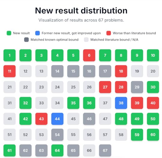
We tested this tool on a large number (67) of different mathematics problems (both solved and unsolved) in analysis, combinatorics, and geometry that we gathered from the literature, and reported our outcomes (both positive and negative) in this paper. In many cases, AlphaEvolve achieves similar results to what an expert user of a traditional optimization software tool might accomplish, for instance in finding more efficient schemes for packing geometric shapes, or locating better candidate functions for some calculus of variations problem, than what was previously known in the literature. But one advantage this tool seems to offer over such custom tools is that of scale, particularly when when studying variants of a problem that we had already tested this tool on, as many of the prompts and verification tools used for one problem could be adapted to also attack similar problems; several examples of this will be discussed below. The following graphic illustrates the performance of AlphaEvolve on this body of problems:
Another advantage of AlphaEvolve was robustness adaptability: it was relatively easy to set up AlphaEvolve to work on a broad array of problems, without extensive need to call on domain knowledge of the specific task in order to tune hyperparameters. In some cases, we found that making such hyperparameters part of the data that AlphaEvolve was prompted to output was better than trying to work out their value in advance, although a small amount of such initial theoretical analysis was helpful. For instance, in calculus of variation problems, one is often faced with the need to specify various discretization parameters in order to estimate a continuous integral, which cannot be computed exactly, by a discretized sum (such as a Riemann sum), which can be evaluated by computer to some desired precision. We found that simply asking AlphaEvolve to specify its own discretization parameters worked quite well (provided we designed the score function to be conservative with regards to the possible impact of the discretization error); see for instance this experiment in locating the best constant in functional inequalities such as the Hausdorff-Young inequality.
A third advantage of AlphaEvolve over traditional optimization methods was the interpretability of many of the solutions provided. For instance, in one of our experiments we sought to find an extremum to a functional inequality such as the Gagliardo–Nirenberg inequality (a variant of the Sobolev inequality). This is a relatively well-behaved optimization problem, and many standard methods can be deployed to obtain near-optimizers that are presented in some numerical format, such as a vector of values on some discretized mesh of the domain. However, when we applied AlphaEvolve to this problem, the tool was able to discover the exact solution (in this case, a Talenti function), and create code that sampled from that function on a discretized mesh to provide the required input for the scoring function we provided (which only accepted discretized inputs, due to the need to compute the score numerically). This code could be inspected by humans to gain more insight as to the nature of the optimizer. (Though in some cases, AlphaEvolve’s code would contain some brute force search, or a call to some existing optimization subroutine in one of the libraries it was given access to, instead of any more elegant description of its output.)
For problems that were sufficiently well-known to be in the training data of the LLM, the LLM component of AlphaEvolve often came up almost immediately with optimal (or near-optimal) solutions. For instance, for variational problems where the gaussian was known to be the extremizer, AlphaEvolve would frequently guess a gaussian candidate during one of the early evolutions, and we would have to obfuscate the problem significantly to try to conceal the connection to the literature in order for AlphaEvolve to experiment with other candidates. AlphaEvolve would also propose similar guesses for other problems for which the extremizer was not known. For instance, we tested this tool on the sum-difference exponents of relevance to the arithmetic Kakeya conjecture, which can be formulated as a variational entropy inequality concerning certain two-dimensional discrete random variables. AlphaEvolve initially proposed some candidates for such variables based on discrete gaussians, which actually worked rather well even if they were not the exact extremizer, and already generated some slight improvements to previous lower bounds on such exponents in the literature. Inspired by this, I was later able to rigorously obtain some theoretical results on the asymptotic behavior on such exponents in the regime where the number of slopes was fixed, but the “rational complexity” of the slopes went to infinity; this will be reported on in a separate paper.
Perhaps unsurprisingly, AlphaEvolve was extremely good at locating “exploits” in the verification code we provided, for instance using degenerate solutions or overly forgiving scoring of approximate solutions to come up with proposed inputs that technically achieved a high score under our provided code, but were not in the spirit of the actual problem. For instance, when we asked it (link under construction) to find configurations to extremal geometry problems such as locating polygons with each vertex having four equidistant other vertices, we initially coded the verifier to accept distances that were equal only up to some high numerical precision, at which point AlphaEvolve promptly placed many of the points in virtually the same location so that the distances they determined were indistinguishable. Because of this, a non-trivial amount of human effort needs to go into designing a non-exploitable verifier, for instance by working with exact arithmetic (or interval arithmetic) instead of floating point arithmetic, and taking conservative worst-case bounds in the presence of uncertanties in measurement to determine the score. For instance, in testing AlphaEvolve against the “moving sofa” problem and its variants, we designed a conservative scoring function that only counted those portions of the sofa that we could definitively prove to stay inside the corridor at all times (not merely the discrete set of times provided by AlphaEvolve to describe the sofa trajectory) to prevent it from exploiting “clipping” type artefacts. Once we did so, it performed quite well, for instance rediscovering the optimal “Gerver sofa” for the original sofa problem, and also discovering new sofa designs for other problem variants, such as a 3D sofa problem.
For well-known open conjectures (e.g., Sidorenko’s conjecture, Sendov’s conjecture, Crouzeix’s conjecture, the ovals problem, etc.), AlphaEvolve generally was able to locate the previously known candidates for optimizers (that are conjectured to be optimal), but did not locate any stronger counterexamples: thus, we did not disprove any major open conjecture. Of course, one obvious possible explanation for this is that these conjectures are in fact true; outside of a few situations where there is a matching “dual” optimization problem, AlphaEvolve can only provide one-sided bounds on such problems and so cannot definitively determine if the conjectural optimizers are in fact the true optimizers. Another potential explanation is that AlphaEvolve essentially tried all the “obvious” constructions that previous researchers working on these problems had also privately experimented with, but did not report due to the negative findings. However, I think there is at least value in using these tools to systematically record negative results (roughly speaking, that a search for “obvious” counterexamples to a conjecture did not disprove the claim), which currently only exist as “folklore” results at best. This seems analogous to the role LLM Deep Research tools could play by systematically recording the results (both positive and negative) of automated literature searches, as a supplement to human literature review which usually reports positive results only. Furthermore, when we shifted attention to less well studied variants of famous conjectures, we were able to find some modest new observations. For instance, while AlphaEvolve only found the standard conjectural extremizer  to Sendov’s conjecture, as well as for variants such as Borcea’s conjecture, Schmeisser’s conjecture, or Smale’s conjecture it did reveal some potential two-parameter extensions to a conjecture of de Bruin and Sharma that had not previously been stated in the literature. (For this problem, we were not directly optimizing some variational scalar quantity, but rather a two-dimensional range of possible values, which we could adapt the AlphaEvolve framework to treat). In the future, I can imagine such tools being a useful “sanity check” when proposing any new conjecture, in that it will become common practice to run one of these tools against such a conjecture to make sure there are no “obvious” counterexamples (while keeping in mind that this is still far from conclusive evidence in favor of such a conjecture).
AlphaEvolve did not perform equally well across different areas of mathematics. When testing the tool on analytic number theory problems, such as that of designing sieve weights for elementary approximations to the prime number theorem, it struggled to take advantage of the number theoretic structure in the problem, even when given suitable expert hints (although such hints have proven useful for other problems). This could potentially be a prompting issue on our end, or perhaps the landscape of number-theoretic optimization problems is less amenable to this sort of LLM-based evolutionary approach. On the other hand, AlphaEvolve does seem to do well when the constructions have some algebraic structure, such as with the finite field Kakeya and Nikodym set problems, which we will turn to shortly.
For many of our experiments we worked with fixed-dimensional problems, such as trying to optimally pack  shapes in a larger shape for a fixed value of . However, we found in some cases that if we asked AlphaEvolve to give code that took parameters such as as input, and tested the output of that code for a suitably sampled set of values of of various sizes, then it could sometimes generalize the constructions it found for small values of this parameter to larger ones; for instance, in the infamous sixth problem of this year’s IMO, it could use this technique to discover the optimal arrangement of tiles, which none of the frontier models could do at the time (although AlphaEvolve has no capability to demonstrate that this arrangement was, in fact, optimal). Another productive use case of this technique was for finding finite field Kakeya and Nikodym sets of small size in low-dimensional vector spaces over finite fields of various sizes. For Kakeya sets in
  , it located the known optimal construction based on quadratic residues in two dimensions, and very slightly beat (by an error term of size
  ) the best construction in three dimensions; this was an algebraic construction (still involving quadratic residues) discovered empirically that we could then prove to be correct by first using Gemini’s “Deep Think” tool to locate an informal proof, which we could then convert into a formalized Lean proof by using Google Deepmind’s “AlphaProof” tool. At one point we thought it had found a construction in four dimensions which achieved a more noticeable improvement (of order
  ) of what we thought was the best known construction, but we subsequently discovered that essentially the same construction had appeared already in a paper of Bukh and Chao, although it still led to a more precise calculation of the error term (to accuracy
  rather than
  , where the error term now involves the Lang-Weil inequality and is unlikely to have a closed form). Perhaps AlphaEvolve had somehow absorbed the Bukh-Chao construction within its training data to accomplish this. However, when we tested the tool on Nikodym sets (which are expected to have asymptotic density , although this remains unproven), it did find some genuinely new constructions of such sets in three dimensions, based on removing quadratic varieties from the entire space. After using “Deep Think” again to analyze these constructions, we found that they were inferior to a purely random construction (which in retrospect was an obvious thing to try); however, they did inspire a hybrid construction in which one removed random quadratic varieties and performed some additional cleanup, which ends up outperforming both the purely algebraic and purely random constructions. This result (with completely human-generated proofs) will appear in a subsequent paper.
September 15, 2025
Smooth numbers and max-entropy
Given a threshold  , a
, a  -smooth number (or -friable number) is a natural number whose prime factors are all at most . We use
  to denote the number of -smooth numbers up to . In studying the asymptotic behavior of , it is customary to write as
  (or as
  ) for some
  . For small values of
  , the behavior is straightforward: for instance if
  , then all numbers up to are automatically -smooth, so

 , the only numbers up to that are not -smooth are the multiples of primes
  between and , so


 , there is an additional correction coming from multiples of two primes between and ; a straightforward inclusion-exclusion argument (which we omit here) eventually gives
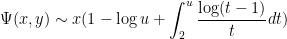
More generally, for any fixed , de Bruijn showed that
 is the Dickman function. This function is a piecewise smooth, decreasing function of , defined by the delay differential equation
 for
for  .
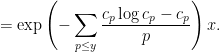
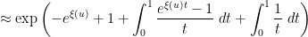
. The asymptotic behavior of as  is rather complicated. Very roughly speaking, it has inverse factorial behavior; there is a general upper bound
 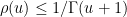 , and a crude asymptotic

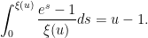
 is the Euler-Mascheroni constant and
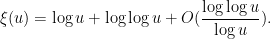
  is defined implicitly by the equation One cannot write in closed form using elementary functions, but one can express it in terms of the Lambert
  function as
 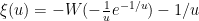 . This is not a particularly enlightening expression, though. A more productive approach is to work with approximations. It is not hard to get the initial approximation
  for large , which can then be re-inserted back into (3) to obtain the more accurate approximation

 to
to
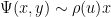
This asymptotic (2) is quite complicated, and so one does not expect there to be any simple argument that could recover it without extensive computation. However, it turns out that one can use a “maximum entropy” to get a reasonably good heuristic approximation to (2), that at least reveals the role of the mysterious function . The purpose of this blog post is to give this heuristic.
Viewing  , the task is to try to count the number of -smooth numbers of magnitude . We will propose a probabilistic model to generate -smooth numbers as follows: for each prime
  , select the prime with an independent probability
  for some coefficient
  , and then multiply all the selected primes together. This will clearly generate a random -smooth number , and by the law of large numbers, the (log-)magnitude of this number should be approximately (where we will be vague about what “
 ” means here), so to obtain a number of magnitude about , we should impose the constraint
The indicator  of the event that divides this number is a Bernoulli random variable with mean , so the Shannon entropy of this random variable is
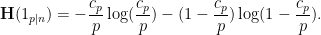
is not too large, then Taylor expansion gives the approximation
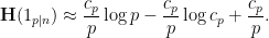
is
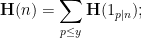
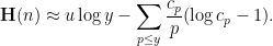
that are typically generated by this random process should be approximately
are chosen to maximize the right-hand side subject to the constraint (5).One could solve this constrained optimization problem directly using Lagrange multipliers, but we simplify things a bit by passing to a continuous limit. We take a continuous ansatz 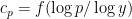 , where
 ![{f: [0,1] \rightarrow {\bf R}}](https://i.gr-assets.com/images/S/compressed.photo.goodreads.com/hostedimages/1758024784i/37228729.png) is a smooth function. Using Mertens’ theorem, the constraint (5) then heuristically becomes and the expression (6) simplifies to So the entropy maximization problem has now been reduced to the problem of minimizing the functional
is a smooth function. Using Mertens’ theorem, the constraint (5) then heuristically becomes and the expression (6) simplifies to So the entropy maximization problem has now been reduced to the problem of minimizing the functional 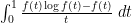 subject to the constraint (7). The astute reader may notice that the integral in (8) might diverge at
  , but we shall ignore this technicality for the sake of the heuristic arguments.
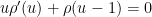
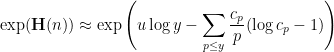
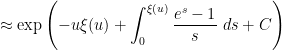
This is a standard calculus of variations problem. The Euler-Lagrange equation for this problem can be easily worked out to be

 ; in other words, the optimal
  should have an exponential form
  . The constraint (7) then becomes

is precisely the mysterious quantity appearing in (2)! The formula (8) can now be evaluated as
 is the divergent constant

 is unrealistic when trying to confine to a single scale ; this comes down ultimately to the subtle differences between the Poisson and Poisson-Dirichlet processes, as discussed in this previous blog post, and is also responsible for the otherwise mysterious
  factor in Mertens’ third theorem; it also morally explains the presence of the same factor in (2). A related issue is that the law of large numbers (4) is not exact, but admits gaussian fluctuations as per the central limit theorem; morally, this is the main cause of the
  prefactor in (2).
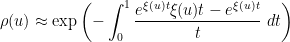
Nevertheless, this demonstrates that the maximum entropy method can achieve a reasonably good heuristic understanding of smooth numbers. In fact we also gain some insight into the “anatomy of integers” of such numbers: the above analysis suggests that a typical -smooth number will be divisible by a given prime  with probability about
  . Thus, for
 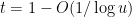 , the probability of being divisible by is elevated by a factor of about
 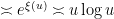 over the baseline probability
  of an arbitrary (non-smooth) number being divisible by ; so (by Mertens’ theorem) a typical -smooth number is actually largely comprised of something like
  prime factors all of size about
  , with the smaller primes contributing a lower order factor. This is in marked contrast with the anatomy of a typical (non-smooth) number , which typically has
  prime factors in each hyperdyadic scale
 ![{[\exp\exp(k), \exp\exp(k+1)]}](https://i.gr-assets.com/images/S/compressed.photo.goodreads.com/hostedimages/1758024785i/37228748.png) in
in ![{[1,n]}](https://i.gr-assets.com/images/S/compressed.photo.goodreads.com/hostedimages/1758024785i/37228749.png) , as per Mertens’ theorem.
, as per Mertens’ theorem.
September 1, 2025
A crowdsourced project to link up erdosproblems.com to the OEIS
Thomas Bloom’s erdosproblems.com site hosts nearly a thousand questions that originated, or were communicated by, Paul Erdős, as well as the current status of these questions (about a third of which are currently solved). The site is now a couple years old, and has been steadily adding features, the most recent of which has been a discussion forum for each individual question. For instance, a discussion I had with Stijn Cambie and Vjeko Kovac on one of these problems recently led to it being solved (and even formalized in Lean!).
A significantly older site is the On-line Encyclopedia of Integer Sequences (OEIS), which records hundreds of thousands of integer sequences that have some mathematician has encountered at some point. It is a highly useful resource, enabling researchers to discover relevant literature for a given problem so long as they can calculate enough of some integer sequence that is “canonically” attached to that problem that they can search for it in the OEIS.
A large fraction of problems in the Erdos problem webpage involve (either explicitly or implicitly) some sort of integer sequence – typically the largest or smallest size  of some -dependent structure (such as a graph of vertices, or a subset of
  ) that obeys a certain property. In some cases, the sequence is already in the OEIS, and is noted in the Erdos problem web page. But in a large number of cases, the sequence either has not yet been entered into the OEIS, or it does appear but has not yet been noted on the Erdos web page.
Thomas Bloom and I are therefore proposing a crowdsourced project to systematically compute the hundreds of sequences associated to the Erdos problems and cross-check them against the OEIS. We have created a github repository to coordinate this process; as a by-product, this repository will also be tracking other relevant statistics about the Erdos problem website, such as the current status of formalizing the statements of these problems in the Formal Conjectures Repository.
The main feature of our repository is a large table recording the current status of each Erdos problem. For instance, Erdos problem #3 is currently listed as open, and additionally has the status of linkage with the OEIS listed as “possible”. This means that there are one or more sequences attached to this problem which *might* already be in the OEIS, or would be suitable for submission to the OEIS. Specifically, if one reads the commentary for that problem, one finds mention of the functions  for
for  , defined as the size of the largest subset of
  without a -term progression. It is likely that several of the sequences
  ,
,  , etc. are in the OEIS, but it is a matter of locating them, either by searching for key words, or by calculating the first few values of these sequences and then looking for a match.
We have set things up so that new contributions (such as the addition of an OEIS number to the table) can be made by a Github pull request, specifically to modify this YAML file. Alternatively, one can create a Github issue for such changes, or simply leave a comment either on the appropriate Erdos problem forum page, or here on this blog.
Many of the sequences do not require advanced mathematical training to compute, and so we hope that this will be a good “citizen mathematics” project that can bring in the broader math-adjacent community to contribute to research-level mathematics problems, by providing experimental data, and potentially locating relevant references or connections that would otherwise be overlooked. This may also be a use case for AI assistance in mathematics through generating code to calculate the sequences in question, although of course one should always stay mindful of potential bugs or hallucinations in any AI-generated code, and find ways to independently verify the output. (But if the AI-generated sequence leads to a match with an existing sequence in the OEIS that is clearly relevant to the problem, then the task has been successfully accomplished, and no AI output needs to be directly incorporated into the database in such cases.)
This is an experimental project, and we may need to adjust the workflow as the project progresses, but we hope that it will be successful and lead to further progress on some fraction of these problems. The comment section of this blog can be used as a general discussion forum for the project, while the github issue page and the erdosproblems.com forum pages can be used for more specialized discussions of specific problems.
August 30, 2025
SLMath announces new research programs
The Simons-Laufer Mathematical Sciences institute, or SLMath (formerly the Mathematical Sciences Research Institute, or MSRI) has recently restructured its program formats, and is now announcing three new research initiatives, whose applications open on Sep 1 2025:
AxIOM (Accelerating Innovation in Mathematics) is a new, month-long research program at SLMath, designed to accelerate innovation and introduce transformative ideas into the mathematical sciences. Programs begin in Spring 2027.PROOF (Promoting Research Opportunities and Open Forums) is a two-week summer program designed to provide research opportunities for U.S.-based mathematicians, statisticians, and their collaborators in the U.S. and abroad, whose ongoing research may have been impacted by factors such as heavy teaching loads, professional isolation, limited access to funding, heavy administrative duties, personal obligations, or other constraints. Programs begin June-July 2026. The priority application deadline for PROOF 2026 is October 12, 2025.Lasting Alliance Through Team Immersion and Collaborative Exploration (LATTICE) is a yearlong program which provides opportunities for U.S. mathematicians to conduct collaborative research on topics at the forefront of the mathematical and statistical sciences. Programs begin June-July 2026. LATTICE 2026 applications are open through February 1, 2026.(Disclosure: I am vice-chair of the board of trustees at SLMath.)
August 10, 2025
Rough numbers between consecutive primes
First things first: due to an abrupt suspension of NSF funding to my home university of UCLA, the Institute of Pure and Applied Mathematics (which had been preliminarily approved for a five-year NSF grant to run the institute) is currently fundraising to ensure continuity of operations during the suspension, with a goal of raising $500,000. Donations can be made at this page. As incoming Director of Special Projects at IPAM, I am grateful for the support (both moral and financial) that we have already received in the last few days, but we are still short of our fundraising goal.
Back to math. Ayla Gafni and I have just uploaded to the arXiv the paper “Rough numbers between consecutive primes“. In this paper we resolve a question of Erdös concerning rough numbers between consecutive gaps, and with the assistance of modern sieve theory calculations, we in fact obtain quite precise asymptotics for the problem. (As a side note, this research was supported by my personal NSF grant which is also currently suspended; I am grateful to recent donations to my own research fund which have helped me complete this research.)
Define a prime gap to be an interval  between consecutive primes. We say that a prime gap contains a rough number if there is an integer
  whose least prime factor is at least the length
  of the gap. For instance, the prime gap
  contains the rough number
  , but the prime gap
  does not (all integers between
  and
and  have a prime factor less than ). The first few for which the
  prime gap contains a rough number are

for which the prime gap does not contain a rough number decays slowly as increases:
Erdös initially thought that all but finitely many prime gaps should contain a rough number, but changed his mind, as per the following quote:
…I am now sure that this is not true and I “almost” have a counterexample. Pillai and Szekeres observed that for every  , a set of
  consecutive integers always contains one which is relatively prime to the others. This is false for
  , the smallest counterexample being
 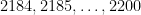 . Consider now the two arithmetic progressions
  and
and  . There certainly will be infinitely many values of for which the progressions simultaneously represent primes; this follows at once from hypothesis H of Schinzel, but cannot at present be proved. These primes are consecutive and give the required counterexample. I expect that this situation is rather exceptional and that the integers for which there is no
  satisfying
  and
and  have density
  .
.
In fact Erdös’s observation can be made simpler: any pair of cousin primes  for
for  (of which is the first example) will produce a prime gap that does not contain any rough numbers.
The latter question of Erdös is listed as problem #682 on Thomas Bloom’s Erdös problems website. In this paper we answer Erdös’s question, and in fact give a rather precise bound for the number of counterexamples:
Theorem 1 (Erdos #682) For, let
be the number of prime gaps
that do not contain a rough number. Then Assuming the Dickson–Hardy–Littlewood prime tuples conjecture, we can improve this to for some (explicitly describable) constant
.
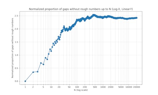
In fact we believe that  , although the formula we have to compute
  converges very slowly. This is (weakly) supported by numerical evidence:
While many questions about prime gaps remain open, the theory of rough numbers is much better understood, thanks to modern sieve theoretic tools such as the fundamental lemma of sieve theory. The main idea is to frame the problem in terms of counting the number of rough numbers in short intervals ![{[x,x+H]}](https://i.gr-assets.com/images/S/compressed.photo.goodreads.com/hostedimages/1731433220i/36158122.png) , where ranges in some dyadic interval
, where ranges in some dyadic interval ![{[X,2X]}](https://i.gr-assets.com/images/S/compressed.photo.goodreads.com/hostedimages/1649687415i/32796876.png) and
and  is a much smaller quantity, such as
  for some
  . Here, one has to tweak the definition of “rough” to mean “no prime factors less than
  ” for some intermediate (e.g.,
 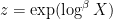 for some
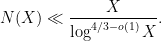
  turns out to be a reasonable choice). These problems are very analogous to the extremely well studied problem of counting primes in short intervals, but one can make more progress without needing powerful conjectures such as the Hardy–Littlewood prime tuples conjecture. In particular, because of the fundamental lemma of sieve theory, one can compute the mean and variance (i.e., the first two moments) of such counts to high accuracy, using in particular some calculations on the mean values of singular series that go back at least to the work of Montgomery from 1970. This second moment analysis turns out to be enough (after optimizing all the parameters) to answer Erdös’s problem with a weaker bound
-tuples, but this was fortunately worked out (in more or less exactly the format we needed) by Montgomery and Soundararajan in 2004. Their focus was establishing a central limit theorem for the distribution of primes in short intervals (conditional on the prime tuples conjecture), but their analysis can be adapted to show (unconditionally) good concentration of measure results for rough numbers in short intervals. A direct application of their estimates improves the upper bound on to
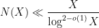
 error. This latter analysis reveals that in fact the dominant contribution to will come with prime gaps of bounded length, of which our understanding is still relatively poor (it was only in 2014 that Yitang Zhang famously showed that infinitely many such gaps exist). At this point we finally have to resort to (a Dickson-type form of) the prime tuples conjecture to get the asymptotic (2).
July 8, 2025
Salem Prize now accepting nominations for 2025
The Salem prize was established in 1968 and named in honor of Raphaël Salem (1898-1963), a mathematician famous notably for his deep study of the links between Fourier series and number theory and for pioneering applications of probabilistic methods to these fields. It was not awarded from 2019-2022, due to both the COVID pandemic and the death of Jean Bourgain who had been almost single-handedly administering the prize, but is now active again, being administered by Akshay Ventakesh and the IAS. I chair the scientific committee for this prize, whose other members are Guy David and Mikhail Sodin. Last year, the prize was awarded to Miguel Walsh and Yilin Wang.
Nominations for the 2025 Salem Prize are now open until September 15th. Nominations should include a CV of the nominee and a nomination letter explaining the significance of the nominee’s work. Supplementary documentation, such as supporting letters of recommendation or key publications, can additionally be provided, but are not required.
Nominees may be individuals from any country or institution. Preference will be given to nominees who have received their PhD in the last ten years, although this rule may be relaxed if there are mitigating personal circumstances, or if there have been few Salem prize winners in recent years. Self-nominations will not be considered, nor are past Prize winners or Scientific Committee members eligible.
The prize does not come with a direct monetary award, but winners will be invited to visit the IAS and to give a lecture associated with the award of the prize.
See also the previous year’s announcement of the Salem prize nomination period.
Terence Tao's Blog

- Terence Tao's profile
- 230 followers

