Brian Potter's Blog

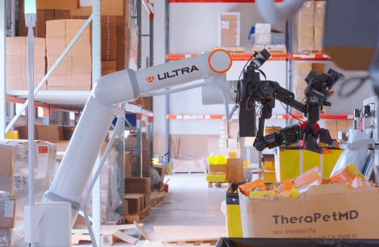Ultra Robotics’ OP1, which mounts a humanoid-ish robot to a larger robot arm, via Jon Schwartz on Twitter.

Welcome to the reading list, a list of news and links related to buildings, infrastructure, and industrial technology. This week we look at transformer steel manufacturing, textile engineering, bringing power plants online quickly, infrasound, and more. Roughly 2/3rds of the reading list is paywalled, so for full access become a paid subscriber.

War in Iran

This week in Strait of Hormuz supply chain issues: a shortage of battery ingredients [Heatmap], the world’s top condom producer plans to raise prices by 20-30% due to petrochemical supply disruption [X], and Lufthansa plans to cut 20,000 flights due to rising jet fuel costs. [UPI]

And it seems like the closure might not be resolved any time soon. It could apparently take up to 6 months to clear the Strait of Hormuz of mines. [Washington Post]

Housing

The Economist on SB-79, and other efforts to stimulate the production of housing in California. “SB 79 rezones state land around busy public-transport stops to allow for taller residential buildings. It also slaps hefty fines on cities that try to deny such buildings a permit. It was amended more than a dozen times to appease rural lawmakers, unions and tenants-rights groups—and it still barely passed the legislature. The bill spent weeks on the governor’s desk, which gave his pro-housing allies the willies and Mr Pratt some hope. But on October 10th Mr Newsom signed the law and delivered a huge win to the ascendant YIMBY (Yes In My Backyard) movement. The passage of SB 79 and more than 40 other housing reforms this year could be a turning point for a state that is crippled by its self-inflicted housing shortage.” [Economist]

Manufacturing

A good Substack post on transformers and why their various components – such as grain oriented electrical steel — are difficult to make. “Producing [GOES] is one of the most demanding metallurgical processes in heavy industry. The slab has to be reheated above 1,350 degrees Celsius to dissolve precipitate inhibitors that later pin grain boundaries, then cold-rolled to the final gauge, and finally decarburized in wet hydrogen to bring the carbon content below 0.003 percent. The entire coil goes into a high-temperature box anneal at 1,200 degrees Celsius for five to seven days, and during that week inside the furnace, through a phenomenon called abnormal grain growth, Goss-oriented grains consume the rest of the matrix and grow to centimeters across a sheet that is barely thicker than a credit card. Premium grades are then laser-scribed in transverse lines to refine the magnetic domains and cut losses by a further ten to fifteen percent. Each step is unforgiving, and a single deviation in composition, atmosphere, or timing ruins the whole coil.” [Frontier Map]

Also on the subject of steel, Did low-quality steel contribute to the sinking of the Titanic? “The steel used in constructing the RMS Titanic was probably the best plain carbon ship plate available in the period of 1909 to 1911, but it would not be acceptable at the present time for any construction purposes and particularly not for ship construction.” [TMS]

Greg Ip of the WSJ claims that the US is in a stealth manufacturing boom, though not one that’s creating jobs. “Since January 2025, manufacturing jobs have indeed fallen by about 100,000 workers, or roughly 0.6%. In the same period, though, manufacturing production rose 2.3%, and manufacturing shipments, unadjusted for inflation, climbed 4.2%.” [WSJ] But Noah Smith argues that no, we aren’t — most manufacturing indicators, once adjusted for inflation, show little to no growth. [Noahpinion]

Chinese electric car manufacturer BYD wants to open 20 dealerships in Canada this year. [GM Authority]

TSMC is apparently delaying using the latest and greatest ASML EUV machines — their High NA machines — because they’re too expensive. [Bloomberg] It’s not clear to me if this is a chance for Intel (who has purchased several High NA machines) to pull ahead, or if Intel overcorrected and made a bad call adopting them.

The changing ownership and subsequent evolution of two different US tool brands, Milwaukee and Craftsman. [Worse on Purpose]

Read more

Not long ago we looked at construction productivity trends for the US and for countries around the world. We found that in the US, and in most other large, wealthy countries, construction productivity is stagnant or declining. Unlike manufacturing and agriculture, or the economy overall, which generally show improving productivity over time, in the field of construction we find that productivity tends to at best stay constant, and at worst decline over time.

Understanding trends in productivity — how much output we get for a given amount of input over time — is useful, but it’s also useful to look at other metrics of construction industry progress. One particularly salient measure is construction costs: how much money it takes to build a house or an office or an apartment building, and how those costs have changed over time. Cost is a good improvement metric because it directly tracks what we actually care about: we would like the costs of building housing, buildings, and infrastructure to fall and become more affordable, and we basically care about more abstract measures like productivity to the extent that they’re a proxy for costs.

Unsurprisingly, when we look at construction costs we see similar trends to what we saw with construction productivity; construction rarely gets any cheaper over time, and construction costs tend to rise at or above the level of overall inflation. As with productivity, we see this when we analyze the data at different levels of granularity, and we see it in both the U.S. and in countries around the world.

Construction cost indexes

Changes in construction cost are generally tracked using cost indexes, measures produced by various organizations which collect and analyze data to try and capture large-scale changes in construction cost. At a high level, there are two broad types of index: output indexes, and input indexes. Output indexes try to measure changes in the cost of finished buildings or infrastructure: how much it costs to build a house, or an office building, or a segment of road over time. Input indexes measure changes in the cost of some basket of construction inputs: the price of different construction tasks, or materials, or labor.

It’s not always straightforward to tell whether an index is an output index or an input index, because exactly how indexes are constructed can be somewhat opaque. An index that initially appears as if it’s an output index, because it apparently tracks changes in a particular type of construction (like new apartment buildings), may actually function more like an input index if it is constructed from price changes in inputs specific to that type of construction. All else being equal, I prefer output indexes to input indexes, because they should more closely track what we actually care about (the cost of finished buildings), and should be less subject to distortion. For instance, the invention of some great cost-saving construction method might not be reflected in an input index that simply tallies up the cost of 10 hours of labor, 100 pounds of steel, and 1 ton of cement (which is how many input indexes are constructed). But in practice output and input indexes tend to track each other quite closely.

Cost indexes are resistant to some of the measurement difficulties that dog productivity metrics, because they’re typically constructed to try and mirror the cost changes of actual buildings. For instance, we’ve previously seen that productivity metrics are dogged by problems of “changes in the output mix” — changes in the type of construction that takes place in a given geography or during a particular collection period can mask actual productivity trends. But the producers of cost indexes will often monitor trends in the construction marketplace, and modify how their index is constructed by weighing some items more heavily and other items less heavily to try and reflect that. We should thus expect them to be more resilient to changing output mix problems.

But in some cases cost indexes share the same measurement issues as productivity metrics. In particular, it can be difficult to adjust cost indexes for quality; a modern building might cost more per square foot, but be built to higher standards or otherwise have higher performance than an older building, which looking only at changes in costs won’t capture. Some indexes, such as the Census Bureau’s Constant Quality Index, try to account for quality changes, but most don’t. (This is in contrast to, say, the Bureau of Labor Statistics’s sector-specific inflation measures, which try to take into account quality changes when calculating inflation trends for things like TVs or new cars.) Indexes that do try to adjust for quality changes likely can’t account for it completely. These issues are somewhat mitigated by the fact that we care about costs as such, and it’s valuable to know how those costs are changing — i.e., even if some proportion of rising costs is due to increased standards and we are getting more bang for our buck, it’s still useful to know how construction costs are changing with respect to other prices. Nonetheless, we should keep this point about quality changes not always being reliably captured mind when we’re looking at cost trends.

To look at trends in U.S. construction costs, we’ll use the following indexes:

Output indexes

The Turner Building Cost Index — Produced by Turner Construction, one of the largest general contractors in the US, this index tracks the price of non-residential buildings by considering such factors as “labor rates and productivity, material prices, and the competitive condition of the marketplace.” This is one of the oldest continuously produced construction cost indexes, going all the way back to 1915.

The Census Bureau’s Single-Family Constant Quality Index — Produced by the US Census Bureau, this index tracks changes in the price of single-family homes, and goes back to 1964.

Handy-Whitman — Produced by Whitman Requardt and Associates, data in this index tracks the cost of building reinforced concrete, brick-lined utility buildings (though there are also other data for other types of buildings). The index is constructed by looking at the price of various inputs (materials, labor, equipment) for these types of buildings, but the relative proportions are adjusted to ensure that they reflect “current construction practice,” so I’m classifying this as an output index. I was able to get data for this index from 1915 to 2002.

Craftsman single-family home costs — Craftsman’s National Construction Estimator, an estimating guide that has been published since the 1950s, includes an estimated cost per square foot to build a “typical” single-family home in the U.S. I was able to get these values going back to 1966.

The National Highway Construction Cost Index — Produced by the U.S. Federal Highway Association, this index tracks the cost of building highways over time, and is based on the price of winning bids for highway construction contracts. This public index goes back to 1915.

Input indexes

E.H. Boeckh Index — Produced by E.H. Boeckh and Associates, this index tracks the cost of a variety of different building types in cities around the U.S., based on “115 elements,” including labor costs, material costs, and tax and insurance elements. (I’m including this in the input indexes because I think it’s basically using the basket-of-inputs approach to construct costs, but depending on how they weighed these elements this might make more sense as an output index.) For many years this index was included in the Survey of Current Business produced by the U.S. Bureau of Economic Analysis. I look at this index for residential construction, for the years 1910 through 1991.

ENR Construction Cost Index — Produced by Engineering News-Record, this index tracks a basket of several different construction inputs — unskilled labor, steel, cement, and wood — the relative proportions of which are periodically adjusted. ENR also produces a virtually identical “Building Cost Index” that replaces unskilled labor with skilled labor. This index has been continuously produced since 1908.

RS Means Historical Cost Index — Produced by the RSMeans estimating company, this index tracks a basket of construction labor, materials and equipment costs. I was able to get data for this index going back to 1953.

Riggleman Index — Produced for an unpublished doctoral dissertation (by Dr. John R. Riggleman) in 1934, this index was made using several other indexes, such as the ENR construction cost index and the American Appraisal Company’s cost index for industrial buildings. This index is primarily useful because it goes back all the way to 1868.

Blank Residential Index — This is another composite index, which uses a weighted basket of construction inputs as well as the E.H. Boeckh index, to track the cost of residential construction. This index is useful because it goes back to 1889.

We’ll compare each of these indexes to the Consumer Price Index (CPI), a common measure of overall inflation. Because the Consumer Price Index only goes back to 1913, for earlier values we’ll use inflation conversion factors produced by Robert Sahr of Oregon State.

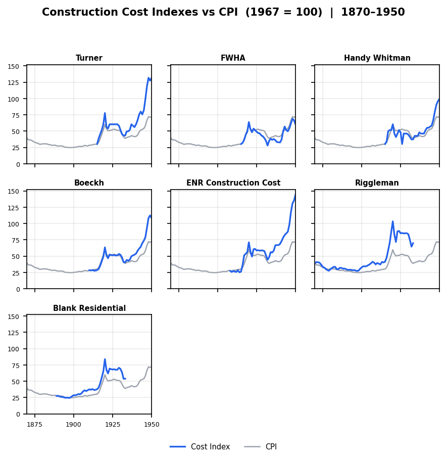
The graphs below show various cost indexes between 1870 and 1950.

And these graphs show cost indexes from 1950 to 2022.

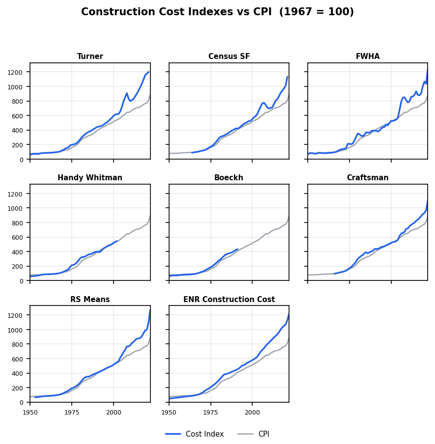
We can see that regardless of time period, and regardless of whether we’re looking at input indexes or output indexes, construction costs are rising roughly as fast as, or faster than, overall inflation. When we looked at productivity trends, we saw that since roughly the 1960s U.S. construction productivity has been stagnant or declining. Cost data suggests that the problem extends even further back, and that U.S. construction costs have virtually never fallen with respect to overall inflation.

These graphs give us a good large-scale view of cost trends for different indices, but it makes it hard to see cost trends over specific time periods. So let’s look at the average annual growth rate for each index over 10-year periods, minus the average growth rate of CPI for the same period. This will let us see how construction costs are changing with respect to inflation over specific periods: positive values mean construction costs are rising faster than inflation, negative means construction costs are rising slower than inflation.

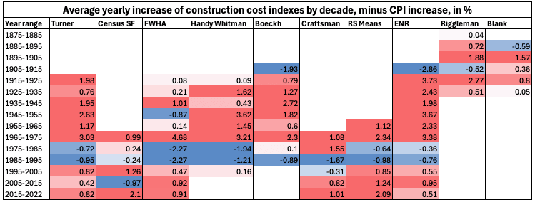
We see that in almost every period of time, construction costs are rising faster than overall inflation for virtually every cost index. The major exception is the period from 1975 to 1995, where most indexes show lower rates of increase or even declines against overall inflation. We also see that historic rates of cost increase seem to be as bad or worse than modern ones. For four of the five 10-year periods between 1915 and 1965, the Turner Cost index rose more than a percentage point faster than overall inflation, whereas for the periods from 1995 to 2025 it rose less than a percentage point.

Construction task costs

As with construction productivity, we can also look at more granular construction cost trends, by looking at how the costs of individual construction tasks have changed. We can do this using construction estimating guides, which provide estimates for the costs of various construction materials and tasks. By looking at the costs of the same, or similar tasks across various versions of estimating guides, we can see how the cost of those tasks are changing.

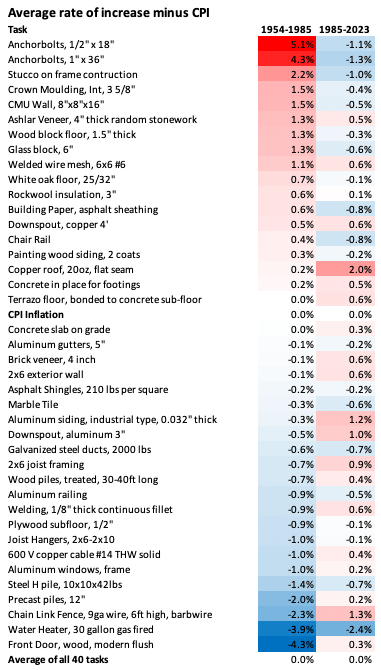
The chart below shows the cost of 40 different construction tasks taken from three different versions of the RSMeans estimating guide published in 1954, 1985, and 2023.

And this chart shows the cost of 20 different construction tasks taken from several different versions of the Craftsman National Construction Estimator published between 1967 and 2016.

!function(){"use strict";window.addEventListener("message",(function(e){if(void 0!==e.data["datawrapper-height"]){var t=document.querySelectorAll("iframe");for(var a in e.data["datawrapper-height"])for(var r=0;r<t.length;r++){if(t[r].contentWindow===e.source)t[r].style.height=e.data["datawrapper-height"][a]+"px"}}}))}();

We can see that cost changes in individual construction tasks aren’t uniform. Some have risen in cost faster than overall inflation; others more slowly. But on average, the cost of these construction tasks has risen at the level of overall inflation. So not only are buildings not getting any cheaper to produce on average, the cost of individual construction tasks isn’t falling either on average, at least for this collection of construction tasks.

There are issues with looking at changes in individual construction tasks. As we noted when we looked at construction productivity, all else being equal we might expect construction to improve by way of introducing new, improved processes, and thus looking at changes in older processes might not reveal very much. In the 19th century, nails got cheaper due to the introduction of new nailmaking processes - replacing hand-made nails with the cut nail process, and then the wire-nail process. If we looked only at improvements in hand-made nails, we might conclude that nails on the market hadn’t gotten any cheaper, even though what actually happened was that an older process had simply been replaced by a newer, better process. I’ve tried to avoid this by using construction tasks that I know are still in use, but this isn’t perfect. Unfortunately, this method may run into an adverse selection problem: picking tasks that appear in many versions of the estimating guide might deliberately select for ones that have been difficult to substitute. Nonetheless, it’s the best method we have for analyzing costs at the granular task level.

We can address this issue the same way we did when we looked at construction productivity, by looking at cost trends in broad categories of tasks. The chart below shows the cost per square foot for 32 categories of tasks required to build a single-family home from Craftsman’s National Construction Estimator. As we can see, task costs generally rise at roughly the same rate that overall home prices rise, and rarely change. (This is sort of mechanical outcome of the fact that task category prices are given as a percentage of overall costs, and for most task categories that percentage has changed little over time, but it’s nevertheless notable.)

Thus, at the level of construction tasks, we also see costs tending to rise at or above the level of overall inflation.

International construction costs

To see whether this trend is also observed internationally, we can look at similar construction cost indexes constructed for other countries. The cost indexes we’ll look at are below:

Eurostat Construction Producer Price Index for Residential Buildings — This cost index, produced by Eurostat for 36 different European countries, tracks the cost changes for residential buildings. (It’s not particularly clear to me how this was constructed: the website merely says that producer price indexes track “the average price development of all goods and related services resulting from that activity.”) For most countries this index goes back to 2000, but for some it goes all the way back to the 1950s.

The U.K.’s BIS construction output price index — This index tracks output prices for several different UK construction sectors (I used values from “All Construction”), going back to 1955. Because this index only goes up to 2011, I supplemented this with the similar Construction Output Price Index from the U.K.’s Office for National Statistics, which began in 2014.

Belgium’s ABEX index — This index tracks the price of building residences in Belgium. The Eurostat Producer Price Index includes data for Belgium, but it only goes back to 2000, whereas the ABEX index goes all the way back to 1914(!).

Japan’s Construction Cost Deflator — This index tracks price changes for several different sectors of Japanese construction, going back to 1960. I used the value for residential construction.

South Korea’s Construction Cost Index — This index tracks the change in construction costs for several different Korean construction sectors, going back to 2000. I used the index for housing construction.

Hong Kong’s Building Works Tender Price Index — Tracks the cost of new buildings in Hong Kong, based on contractor bids. Goes back to 1970.

Taiwan’s Construction Price Index — This index tracks the changes in construction costs in Taiwan, and is based on the prices of 115 different construction inputs. It goes back to 1991.

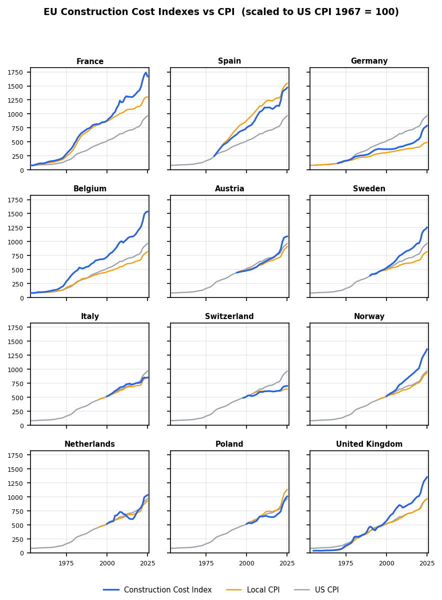
The graphs below show each of these indexes against the consumer price index for 12 major European countries, as well as the U.S. consumer price index.

And this graph shows construction cost trends for Asian countries.

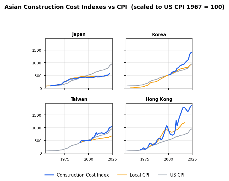
We see the same pattern that we saw with U.S. construction cost indexes: construction costs nearly always rise at, or faster than, the level of overall inflation in the country.

We can also see this if we look at changes in construction cost minus changes in consumer price index in 10-year buckets, as we did for U.S. construction costs. The chart below shows decade-by-decade changes in construction cost minus CPI for 41 different European and Asian countries (including lots of smaller and poorer countries that I didn’t include on the above graphs).

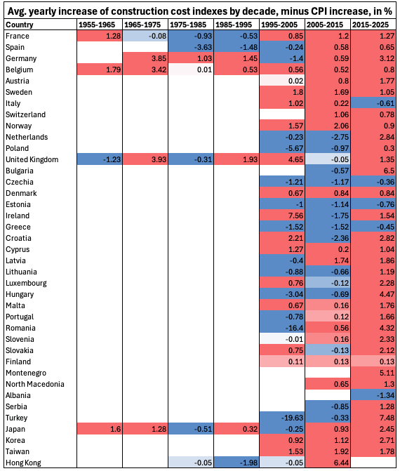
There’s somewhat more blue on this chart than in the US construction costs, but we can still see costs are, more often than not, rising faster than overall inflation.

Conclusion

When we looked at trends in construction productivity — how much construction output we get for a given amount of input — we saw that it’s mostly either relatively unchanging, or declining over time. We saw this in the U.S. using a variety of different metrics of varying granularity, and we saw it in most other wealthy countries. With construction costs — how much construction output we get for a given amount of currency — we see something similar. Construction costs tend to rise at, or above, the level of overall inflation, and it rarely (if ever) gets cheaper to build houses, offices, or other buildings. We see this in the U.S. with a variety of different metrics, and we see it in countries around the world. With stagnant construction productivity, we could date the problem as far back as roughly the 1960s. With construction costs, we can push the problem back even further: outside of a few windows of time, construction costs have virtually never fallen with respect to overall inflation.

Path Robotics’ welding quadruped, via Nima Gard on Twitter.

Welcome to the reading list, a weekly roundup of news and links related to buildings, infrastructure, and industrial technology. This week we look at a quadruped welding robot, the China Shock 2.0, transformer startups, China’s mysteriously moving satellites, and more. Roughly 2/3rds of the reading list is paywalled, so for full access become a paid subscriber.

No essay this week, but working on a more involved piece about construction costs in the US and around the world that should be out next week.

War in Iran

The US has blockaded the Strait of Hormuz, preventing Iranian ships from transiting the strait. “On Monday, the United States imposed its own naval blockade, intent on ending Iran’s dominance of the waterway and cutting off its oil income by blocking all traffic to and from its ports…Since the U.S. blockade took effect, no ships linked to Iran have been spotted leaving the region, according to the vessel‑tracking company Kpler.” [NYT] Negotiations between the US and Iran are apparently ongoing, but the strait seems to be closed as of this writing. [BBC]

The strait’s closure continues to disrupt supply chains around the world: Russia has imposed export controls on helium [Reuters], airlines continue to be squeezed by the high cost of jet fuel [WSJ], and a Japanese bathroom manufacturer shut down production due to a lack of glue. [Nikkei Asia]

Thanks to the war, GPS signals are being jammed across the region. One consequence? Food delivery drivers are having trouble delivering their orders. [Rest of World]

The Saudi East-West oil pipeline being used to bypass the Strait of Hormuz had been damaged by an Iranian drone attack, but now appears to be back online. [Reuters]

Housing

Homeownership rates by state in the US. Some of these figures surprise me: it’s not hard to understand why California and New York might have low homeownership rates due to the high costs of real estate, but Georgia, Texas, and North Dakota being on the low end and West Virginia being on the high end are more surprising to me. [X]

Also on the subject of home ownership, the White House released a report on “Rebuilding and Protecting the American Dream of Homeownership.” It looks at various causes of high housing prices in the US, and concludes with some recommendations for states and local jurisdictions to reduce housing costs:

Unleashing manufacturing innovation: “...align codes with accepted standards for modular, prefabricated, panelized, and other off-site built housing.”

Streamlining the stages of homebuilding: “...create a fast-track process for all housing developments that features capped timelines and permit fees, appropriate and justifiable impact fees, third-party inspections, and an expedited appeal process that ensures faster and less arbitrary dispute resolution.”

Protecting consumer choice and private property rights: “...curtail gratuitous mandates that restrict housing supply, such as restrictions on the number of units that can be built in any given time period, costly green energy building requirements, and discriminatory labor rules.”

Most of these seem like reasonable ideas to me. [White House]

Manufacturing

The Pentagon wants to get US auto manufacturers involved in weapons production, as the wars in Ukraine and Iran run down ordnance stockpiles. This was widely done during WWII, but it’s not obvious how easily today’s car manufacturers could pivot. [WSJ]

Also on the subject of weapons manufacturing, Detroit is angling to be the epicenter of a new US drone manufacturing industry. “Thanks to ramped-up military spending on drones and their proliferation in civilian uses, the market for American-made unmanned aerial systems is expected to grow to more than $50 billion by 2030, from $5 billion this year…Companies are scrambling to build a supply chain from scratch, and states are vying to be at the center of it. In July, Gov. Gretchen Whitmer of Michigan, a Democrat, issued an executive directive calling for a statewide effort to scale up “advanced air mobility” manufacturing, which includes drones and electric planes.” [NYT]

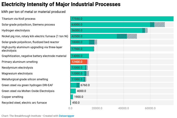
Tulsa, Oklahoma is building the first aluminum smelter built in the US in 50 years, which would double(!) US smelting capacity. [WSJ] Related, this Breakthrough Institute Piece on aluminum and China’s manufacturing prowess has an interesting graphic showing which materials require the most electricity to produce. Titanium requires way more electricity, and electric arc steel requires way less electricity, than I realized. [Breakthrough]

When I looked at welding automation a few years ago, one of the startups I highlighted trying to push automated welding forward was Path Robotics, which at the time was developing a system that could automatically plan out a welding path based on computer vision and a CAD model it had been provided. Now the company just introduced an automated welding system mounted to a robot dog. The utility of this isn’t amazingly obvious to me — I think most welding is probably done in repeatable locations where the dog is unnecessary, in locations that would be tricky for a dog to access, or require some kind of workholding that this doesn’t seem equipped with — but it’s cool nonetheless. [X]

A cool short video clip showing manufacturing of wooden propellers using Blanchard-style pattern-tracing lathes. [X]

Slate Auto, the Jeff Bezos-backed startup that wants to build a no-frills EV truck, raised another $650 million, bringing its total funding to $1.4 billion. [TechCrunch]

Read more

Antarctic snow cruiser circa 1939, via Historyland.

Welcome to the reading list, a weekly roundup of news and links related to buildings, infrastructure, and industrial technology. This week we look at whether the Strait of Hormuz is open yet, building code cost benefit analysis, Intel joining Terafab, sponge cities, and more. Roughly 2/3rds of the reading list is paywalled, so for full access become a paid subscriber.

War in Iran

A two-week ceasefire between the US and Iran was announced earlier this week, in exchange for Iran opening the Strait of Hormuz. [BBC] But despite the agreement, so far Iran seems to have kept the Strait closed. [AP News]

“Is Hormuz Open Yet?” is a website for tracking the status of ship crossings in the Strait of Hormuz. [Is Hormuz Open Yet?]

Prior to the cease fire Iran was apparently attempting cyberattacks on US infrastructure. “Iran-affiliated advanced persistent threat (APT) actors are conducting exploitation activity targeting internet-facing operational technology (OT) devices, including programmable logic controllers (PLCs) manufactured by Rockwell Automation/Allen-Bradley. This activity has led to PLC disruptions across several U.S. critical infrastructure sectors through malicious interactions with the project file and manipulation of data on human machine interface (HMI) and supervisory control and data acquisition (SCADA) displays, resulting in operational disruption and financial loss.” [CISA] [LA Times]

Prior to the cease fire Iran threatened to target OpenAI’s Stargate data center in Abu Dhabi. [The Verge] And Microsoft is apparently considering designing more resilient data centers in high-risk areas. [The Register]

This week Iranian drone attacks targeted Saudi Arabia’s Jubail petrochemical complex, [Reuters] UAE’s Habshan gas facility [Al Jazeera], and power and desalination plants in Kuwait. [Al Jazeera]

The US supposedly located the weapons officer of the F-15E shot down in Iran using “Ghost Murmur,” a tool that allegedly uses “long-range quantum magnetometry to find the electromagnetic signal of a human heartbeat.” [NY Post]

Housing

A paper from UCLA’s Lewis Center takes a look at the process of building code development, and notes that provisions added to the building code rarely undergo any sort of cost-benefit analysis. “For example, when a fire marshall in Glendale, Arizona proposed two decades ago that US elevators be required to be larger than international standards to accommodate a 7-ft stretcher lying flat, the cost impact was reported as “none” (Grabar 2025). Today, it is among the reasons that a basic four-stop elevator in New York City costs about $158,000, compared to $36,000 in Switzerland (Smith 2024). These costs are ultimately borne not only as more expensive elevator amenitized buildings, but in the prevalence of newly constructed five- and six-story walk-ups in the US, which are inaccessible to many elderly and disabled tenants and are unheard of in most high-income countries (Smith 2024).” [Escholarship] Building code cost-benefit analysis was one of the points of advocacy from the White House Executive order a few weeks ago. [White House]

Most single-family homes in the US are built to the requirements of the (inaccurately named) International Residential Code. But apartment buildings are built to the somewhat-more-strict International Building Code, even small, house-like apartment buildings like triplexes. The Congress for New Urbanism proposes expanding the IRC to cover small apartment buildings as well. [CNU]

British building standards apparently recommend that windows be sized so that they’re cleanable from the inside by “95% of the elderly female population, without the need for stretching;” if this (non-binding, but often followed in practice) recommendation is followed, the result is extremely tiny windows. [X]

IFP’s infrastructure team has a good piece on how the build-to-rent provisions in the Senate’s ROAD to housing act would dramatically reduce new home construction in the US. (I’m a member of IFP’s infrastructure team, but didn’t help write this piece.) “At President Trump’s request, the Senate acted to prohibit institutional investors from buying up single-family homes. This provision is captured in Section 901 of 21st Century ROAD, “Homes are for people, not corporations.” But while the White House’s Executive Order and proposed legislative text would ban institutional investors from purchasing existing single-family homes, they explicitly protected investor financing of new rental homes. The Senate’s Section 901 goes further: it establishes a disposition requirement for investors to sell their newly built one- and two-family homes within a fixed period, discouraging investment in new rental homes and decreasing housing supply. The last-minute inclusion of Section 901 with this disposition requirement has jeopardized the overall package and fueled calls for a fix in the House. The housing industry, the pro-housing advocacy community, and both Democrats and Republicans in the House and Senate, as well as members of the administration, have voiced opposition to the section as written.” [IFP]

Read more

The war in Iran, and the subsequent closure of the Strait of Hormuz, has unfortunately made us all familiar with details of the petroleum supply chain that we could formerly happily ignore. Every day we get some new story about some good or service that depends on Middle East petroleum and the production of which has been disrupted by the war. Fertilizer production, plastics, aluminum, the list goes on.

One such supply chain that’s suddenly getting a lot of attention is helium. Helium is produced as a byproduct of natural gas extraction: it collects in the same underground pockets that natural gas collects in. Qatar is responsible for roughly 1/3rd of the world’s supply of helium, which was formerly transported through the Strait of Hormuz in specialized containers. Thanks to the closure of the strait, helium prices have spiked, suppliers are declaring force majeure, and businesses are scrambling to deal with looming shortages. (For many years the US government maintained a strategic helium reserve, but this was sold off in 2024.)

What I find interesting about helium is that in many cases, it’s very hard to substitute for. Helium has a unique set of properties — in particular, it has a lower melting point and boiling point than any other element — and technologies and processes that rely on those properties can’t easily switch to some other material.

Helium production

Helium is the second lightest element in the periodic table (after hydrogen), and the second most common element in the universe (also after hydrogen). But while helium is very common on a cosmic scale, here on earth it’s not so easy to get. Because helium is so light, it rises to the very top of the atmosphere, where it eventually escapes into space.1 So essentially all helium used by modern civilization comes from underground.

Helium is produced via the radioactive decay of elements like uranium and thorium, and it collects in underground pockets of natural gas. This source of helium was first discovered in the US in 1903, when a natural gas well in Kansas produced a geyser of gas that refused to burn. Scientists at the University of Kansas eventually determined that this was due to the presence of helium. Like petroleum, helium has collected in these pockets over the course of millions of years, and thus (like petroleum) there’s a limited supply of underground helium that can be extracted. As with petroleum, people are often worried that we’re running out of it.

Because helium is a byproduct of natural gas extraction, and because only some natural gas fields have helium in appreciable quantities, a small number of countries are responsible for the world’s supply of helium. The US and Qatar together produce around 2/3rds of the world’s helium supply. Russia, Algeria, Canada, China, and Poland produce most of the remaining balance.

!function(){"use strict";window.addEventListener("message",(function(e){if(void 0!==e.data["datawrapper-height"]){var t=document.querySelectorAll("iframe");for(var a in e.data["datawrapper-height"])for(var r=0;r<t.length;r++){if(t[r].contentWindow===e.source)t[r].style.height=e.data["datawrapper-height"][a]+"px"}}}))}();!function(){"use strict";window.addEventListener("message",(function(e){if(void 0!==e.data["datawrapper-height"]){var t=document.querySelectorAll("iframe");for(var a in e.data["datawrapper-height"])for(var r=0;r<t.length;r++){if(t[r].contentWindow===e.source)t[r].style.height=e.data["datawrapper-height"][a]+"px"}}}))}();

Elemental helium has a few different useful properties. The most important one is that, thanks to the small size and completely filled outer electron shell of helium atoms, helium has a lower boiling point than any other element. Liquid helium boils at just 4.2 kelvin (-452 degrees Fahrenheit). By comparison, liquid hydrogen boils at 20 K, and liquid nitrogen boils at a positively balmy 77 K.

!function(){"use strict";window.addEventListener("message",(function(e){if(void 0!==e.data["datawrapper-height"]){var t=document.querySelectorAll("iframe");for(var a in e.data["datawrapper-height"])for(var r=0;r<t.length;r++){if(t[r].contentWindow===e.source)t[r].style.height=e.data["datawrapper-height"][a]+"px"}}}))}();

Its low boiling point makes helium very useful for getting something really, really cold. When a liquid boils, it transforms into a gas, and during this process it will pull energy from its surroundings due to evaporative cooling. This is why your body sweats: to cool you down as the liquid evaporates. When a liquid has a very low boiling point, this heat extraction happens at a very low temperature. Helium also stays a liquid at much lower temperatures than other elements. Nitrogen freezes solid at 63 K, and hydrogen freezes at 14K, but at atmospheric pressure helium stays a liquid all the way to absolute zero. If you need to cool something to just a few degrees above absolute zero, liquid helium is essentially the only practical way to do that.

Helium also has a few other useful properties. As we noted, helium is very light: it will naturally rise in the atmosphere, which makes it useful as a lifting gas. Thanks to its filled outer electron shell, it is inert, and won’t react with other materials. Helium also has high thermal conductivity — at room temperature, helium can move heat about six times better than air.

The uses of helium

The world uses around 180 million cubic meters of helium each year. (This sounds like a lot, but it’s just 0.11% of the 159 billion cubic meters of nitrogen the world uses each year, and 0.004% of the over 4 trillion cubic meters of natural gas that the world uses each year.) But while it’s not used in enormous quantities compared to some other gases, helium is nevertheless quite important. Different industries make use of helium’s properties in different ways, and while in some cases there are reasonable substitutes for helium, in most cases helium has no practical replacement.

!function(){"use strict";window.addEventListener("message",(function(e){if(void 0!==e.data["datawrapper-height"]){var t=document.querySelectorAll("iframe");for(var a in e.data["datawrapper-height"])for(var r=0;r<t.length;r++){if(t[r].contentWindow===e.source)t[r].style.height=e.data["datawrapper-height"][a]+"px"}}}))}();MRI machines

Some of the biggest consumers of helium are MRI machine operators, which consume around 17% of the helium used in the US. MRI machines work by creating very strong magnetic fields, which change the orientation of hydrogen atoms in tissues in your body. A pulse of radio waves is then sent into your body, which temporarily disrupts this orientation. When the pulse stops, different types of tissue return to their alignment with the magnetic field at different rates, and that rate of change can be measured and converted into a picture of the interior of the body. The strong magnetic fields in MRI machines are created by superconducting magnets: when some materials get cold enough, they drop to zero electrical resistance, which makes it possible to put enormous amounts of electrical current through them and create extremely strong magnetic fields.2 The vast majority of MRI machines used today use superconducting magnets made from niobium-titanium (NbTi), which becomes superconducting at 9.2 degrees above absolute zero. This is well below the boiling point of any other coolant, making liquid helium the only practical option for cooling the magnets. A handful of MRI machines have been built using higher-temperature superconductors that don’t require helium cooling, but the vast majority of the 50,000 existing MRI machines in the world require helium.

The helium consumption of MRI machines has fallen drastically over time. Early MRI machines would lose helium at a rate of around 0.4 liters per hour, requiring large tanks of 1000-2000 liters that needed to be refilled every few months. (It’s notoriously difficult to prevent gaseous helium from leaking out of containers, which is why helium is also often used for leak detection.) But modern MRI machines are “zero boil-off,” which essentially never need to be recharged with helium. As these machines take up more market share, the helium requirements of MRI machines can be expected to fall. But for the foreseeable future, MRI will remain a substantial source of demand.

Semiconductors

Another major consumer of helium is the semiconductor industry, which uses around 25% of the helium worldwide, and around 10% of the helium in the US.3 As with MRI machines, helium is used to cool superconducting magnets, which are used to increase the purity of silicon ingots grown using the Czochralski method. Helium is also used as a coolant in some production processes, as well as a non-reactive gas to flush out some containers, for leak detection, and for a variety of other uses. A 2023 report from the Semiconductor Industry Association noted that helium was used “as a carrier gas, in energy and heat transfer with speed and precision, in reaction mediation, for back side and load lock cooling, in photolithography, in vacuum chambers, and for cleaning.” The same report notes that for many of these uses, helium has no substitute.

Unlike MRI machines, which have used less and less helium over time, helium usage in the semiconductor industry seems to be trending up: some sources claim that helium consumed by the semiconductor industry is expected to rise by a factor of five by 2035. This seems to be in part due to the development of DUV and EUV semiconductor lithography machines, which require helium to function. Unlike many other gases, helium absorbs almost no EUV radiation, which (as I understand it) makes it hard to substitute for helium in EUV machines.

Fiber optics

Helium is also used in the manufacturing of fiber optic cable. Optical cable is made with an inner core of glass, surrounded by an outer “sleeve” of glass with a different index of refraction. This keeps photons within the inner core via the phenomenon of total internal reflection. During the manufacturing process, helium is used as a coolant when the outer “sleeve” is being deposited onto the core — with any other atmosphere, bubbles form between the two layers of glass. Roughly 5-6% of helium worldwide is used for the production of optical fiber, and there’s no known alternative.

Purging gas

Other than semiconductor manufacturing, other industries (particularly the aerospace industry) use helium as a “purge gas” to clean out containers. Cleaning out a tank of liquid hydrogen, often used as a liquid rocket fuel, requires a gas with a boiling point low enough that it won’t freeze when it contacts the hydrogen. Cleaning a tank of liquid oxygen doesn’t require a gas with quite as low a boiling point, but it is best to use an inert gas to reduce the chance of it reacting with the highly reactive oxygen. Aerospace purging makes up around 7% of US helium consumption. Around half of that is used by NASA, which is the single biggest user of helium in the US.

Lifting gas

Because helium is lighter than air, it’s also used as a lifting gas in balloons and lighter-than-air airships as an alternative to the highly flammable hydrogen. Each Goodyear Blimp, for instance, uses around 300,000 cubic feet of helium. Around 18% of the helium consumed in the US is as a lifting gas.

Scientific research and instruments

Helium is also widely used in scientific research. Much of this is for keeping things cold: superconducting magnets, such as those used in the Large Hadron Collider, typically require helium, as do the superconducting elements in SQUIDs, which are highly sensitive magnetic field detectors. Helium is also used in mass spectrometers, which are used for, among other things, detecting microscopic leaks in containers.

This is a major category of use in the US; roughly 22% of its helium consumption goes to “analytical, engineering, lab, science, and specialty gases.”

Welding

In the US, helium is also used for welding: its high thermal conductivity and its inertness make helium an excellent shielding gas, which prevents the pool of molten metal from being contaminated before it cools. In the US, welding makes up roughly 8% of helium use, but elsewhere in the world, it’s more common to use other shielding gases like argon.

Diving

Helium is also used for breathing gas in deep sea commercial diving. At depths beyond 30 meters, breathing nitrogen (which makes up 78% of normal air) causes nitrogen narcosis, and diving beyond this depth is done using gas mixes that replace part of the nitrogen for helium. Roughly 5% of helium consumed in the US goes towards diving.

Helium for diving is difficult to substitute for. Virtually every other breathable gas except for possibly neon causes some degree of narcosis, and neon is heavier than helium, making breathing more difficult.

Conclusion

For some of these applications, it’s possible to substitute helium with other materials. There are other shielding gases, such as argon, that can be used for welding, and other lifting gases, such as hydrogen, that can be used for balloons or airships. In other applications, it’s possible to dramatically reduce the consumption of helium via recycling systems or other methods designed to reduce its use. As we’ve noted, this has occurred with MRI machines, where modern ones use far less helium than their predecessors. And it seems to have happened with aerospace purging. A 2010 report from the National Academies of Sciences notes that if NASA and the Department of Defense were sufficiently motivated, they could dramatically reduce their helium consumption by recycling it. Since then, aerospace use of helium has fallen from 18.2 million cubic meters (26% of total US consumption) to 4 million cubic meters (7% of total US consumption). But the United States Geological Survey notes that most helium in the US is still unrecycled, and there’s lots of opportunity to dramatically reduce helium usage with various recapture and recycling systems. Many of these systems are capable of reducing helium consumption by 90% or more.

But “reducing” doesn’t mean “eliminating,” and it’s interesting to me how in so many cases there doesn’t seem to be any good substitute for helium.

1

Though thanks to circulation in the air, the helium concentration below the turbopause is roughly constant, about 5 parts per million.

2

If the magnets get too warm, the sudden loss of superconductivity, called a “quench,” can damage or destroy the magnets due to the heat generated from the now-present electrical resistance.

3

I estimated this by subtracting the 5-6% of helium used globally by the fiber optic industry from the 15% of helium used by “semiconductors and fiber optics” from the United States Geological Survey report on helium.

UAE cabinet meeting room, via Camski.

Welcome to the reading list, a weekly roundup of news and links related to buildings, infrastructure, and industrial technology. This week we look at aluminum disruptions, the EV rust belt, the ongoing transformer shortage, SpaceX’s IPO, and more. Roughly 2/3rds of the reading list is paywalled, so for full access become a paid subscriber.

War in Iran

The world’s largest aluminum smelter in Bahrain was hit by an Iranian drone, bringing production offline. [Bloomberg] Other aluminum smelters in the area have cut production due to inability to ship through the Strait. This, in turn, has forced various EV manufacturers to cut production. “Gulf smelters that supply Toyota, Nissan, BMW, parts makers for Mercedes-Benz, South Korea’s Hyundai Mobis and hundreds of other automotive customers worldwide are defaulting on contracts or closing down. The U.S.-Iran war has effectively shut the Strait of Hormuz to commercial shipping, cutting off one of the largest flows of automotive-grade aluminum.” [Rest of World]

Israel bombed two Iranian steel factories. [NYT] The US bombed an Iranian bridge that was one of the largest in the Middle East. [BBC] And another Amazon data center was damaged by an Iranian drone. [Reuters]

The Philippines declares a National Energy Emergency. [Reuters] And Germany considers ramping up coal power to avert an energy crisis. [Politico]

Helium production in Qatar, which is responsible for roughly 1/3rd of the world’s supply, has been shut down. [NYT] We’ve previously noted that helium is a critical input for semiconductor manufacturing and MRI machines, but it’s apparently also crucial for mass spectrometers used in science labs. [X]

The world is running out of ways to deal with the disruption to oil supply that don’t involve using less oil. “In the first days of this war, the strait’s closure meant the immediate loss of 20 million daily barrels of crude and refined products. The industry went to work, activating a first layer of defense: using up stocks. The second layer came soon after as Saudi Arabia and the United Arab Emirates rerouted some exports using bypass pipelines to Red Sea and Gulf of Oman ports. The third defense came from politicians. The richest nations tapped their strategic reserves, injecting millions of barrels into the market. US President Donald Trump also made constant — and effective — verbal interventions. His jawboning about the chance of an end to the fighting helped tame panic buying.” [Bloomberg]

Italy denied US military aircraft permission to land at a base in Sicily for operations against Iran. [Bloomberg]

Because Iranian ships can traverse the Strait of Hormuz freely, Iran is actually making more money from oil sales than it was prior to the war. “Iran is now earning nearly twice as much from oil sales each day as it did before American and Israeli bombs started falling on February 28th. It may be pummelled on the battlefield, but the regime is winning the energy war.” [The Economist]

Housing

25 housing researchers signed an open letter opposing the provisions in the ROAD to housing act recently passed by the Senate that would limit build-to-rent housing. “If passed, the seven-year disposition requirement would result in a decline of more than 7% of single-family home completions and 18% of rental completions, according to analysis from Laurie Goodman and Jim Parrott at the Urban Institute, a Washington, D.C.-based think tank.” [Multifamily Dive]

Work on what would be the tallest mass timber building in the US (in Milwaukee of all places), has apparently stopped, and the project is facing foreclosure. [Multifamily Dive]

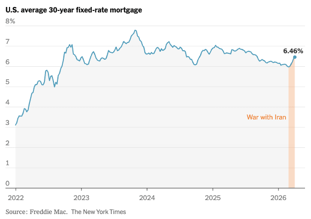
Mortgage rates had been steadily, if slowly, declining over the last year, but since the beginning of the war in Iran they’ve ticked back up. [NYT]

Japanese corporations keep buying US homebuilders. “Japanese builders have announced or closed acquisitions of 23 U.S. single-family home builders since 2020, more than double the number from 2013 to 2019. That doesn’t include the multifamily developers and construction-supply companies they have also bought. By some estimates, Japanese builders are now set to own about 6% of the U.S. home-construction market.” [WSJ]

Read more

I spend a lot of time reading about the nature of technological progress, and I’ve found that the literature on technology is somewhat uneven. If you want to learn about how some particular technology came into existence, there’s often very good resources available. Most major inventions, and many not-so-major ones, have a decent book written about them. Some of my favorites are Crystal Fire (about the invention of the transistor), Copies in Seconds (about the early history of Xerox), and High-Speed Dreams (about early efforts to build a supersonic airliner).

But if you’re trying to understand the nature of technological progress more generally, the range of good options narrows significantly. There’s probably not more than ten or twenty folks who have studied the nature of technological progress itself and whose work I think is worth reading.

One such researcher is Brian Arthur, an economist at the Santa Fe Institute.1 Arthur is the author of an extremely good book about the nature of technology (called, appropriately, “The Nature of Technology,”) which I often return to. He’s also the co-author, along with Wolfgang Polak, of an interesting 2006 paper, “The Evolution of Technology within a Simple Computer Model,” that I think is worth highlighting. In this paper Arthur evolves various boolean logic circuits (circuits that take ones and zeroes as inputs and give ones and zeroes as outputs) by starting with simple building blocks and gradually building up more and more complex functions (such as a circuit that can add two eight-bit numbers together).

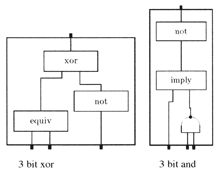Logic circuits invented by Arthur’s simulation.

I wanted to highlight this paper because I think it sheds some light on the nature of technological progress, but also because the paper does a somewhat poor job of articulating the most important takeaways. Some of what the paper focuses on — like the mechanics of how one technology gets replaced by a superior technology — I don’t actually think are particularly illuminating. By contrast, what I think is the most important aspect of the paper — how creating some new technology requires successfully navigating enormous search spaces — is only touched on vaguely and obliquely. But with a little additional work, we can flesh out and strengthen some of these ideas. And when we look a little closer, we find what the paper is really showing us is that finding some new technology is a question of efficiently acquiring information.

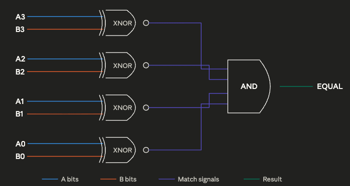
Outline of the paper

The basic design of the experiment is simple: run a simulation that randomly generates various boolean logic circuits and analyze the sort of circuits that the simulation generates. Boolean logic circuits are collections of various functions (such as AND, OR, NOT, EQUAL) that perform some particular operation on binary numbers. The logic circuit below, for instance, determines whether two 4-bit numbers are equal using four exclusive nor (XNOR) gates, which output a 1 if both inputs are identical, and a 4-way AND gate, which outputs a 1 if all inputs are 1. Boolean logic circuits are important because they’re how computers are built: a modern computer does its computation by way of billions and billions of transistors arranged in various logic circuits.

The simulation works by starting with three basic circuit elements that can be included in the randomly generated circuits: the Not And (NAND) gate (which outputs 0 if both inputs are 1, and 1 otherwise), and two CONST elements which always output either 1 or 0. The NAND gate is particularly important because NAND is functionally complete; any boolean logic circuit can be built through the proper arrangement of NAND gates.

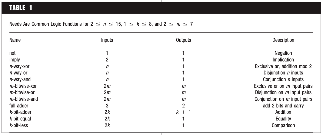
Using these starting elements, the simulation tries to build up towards higher-level logical functions. Some of these goals, such as creating the OR, AND, and exclusive-or (XOR) functions, are simple, and can be completed with just a few starting elements. Others are extremely complex, and require dozens of starting elements to implement: an 8-bit adder, for instance, requires 68 properly arranged NAND gates.

To achieve these goals, during each iteration the simulation randomly combines several circuit elements — which at the beginning are just NAND, one, and zero. It randomly selects between two and 12 components, wires them together randomly, and looks to see if the outputs of the resulting circuit achieve any of its goals. If it has — if, by chance, the random combination of elements has created an AND function, or an XOR function, or any of its other goals — that goal is marked as fulfilled, and circuit that fulfills it gets “encapsulated,” added to the pool of possible circuit elements. Once the simulation finds an arrangement of NAND components that produces AND and OR, for instance, those AND and OR arrangements get added to the pool of circuit elements with NAND and the two CONSTS. Future iterations thus might accidentally stumble across XOR by combining AND, OR, and NAND.

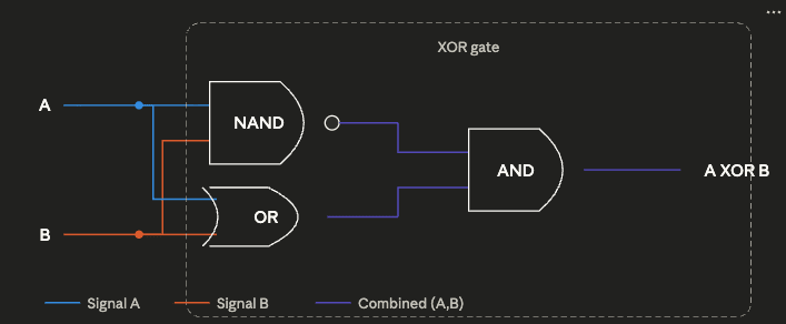An XOR gate made from a NAND, an OR, and an AND gate.

Because finding an exact match for a given goal might be hard, especially as goals get more complex, the simulation will also add a given circuit to the pool of usable components if it partially fulfills a goal, as long as it does a better job of meeting that goal than any existing circuit. Circuits that partially meet some goal (such as a 4-bit adder that gets just the last digit wrong) are similarly used as components that can be recombined with other elements. So the simulation might try wiring up our partly-correct 4-bit adder with other elements (NAND, OR, etc.) to see what it gets; maybe it finds another mini-circuit that can correct that last digit.

Over time, the pool of circuit elements that the simulation randomly draws from grows larger and larger, filled both with circuits that completely satisfy various goals and some partly-working circuits. A circuit can also get added to the pool if it’s less expensive — uses fewer components — than existing circuits for that goal. So if the simulation has a 2-bit adder made from 10 components, but stumbles across a 2-bit adder made from 8 components, the 8-component adder will replace the 10 component one.

When the simulation is run, it begins randomly combining components, which at the beginning are just NAND, one, and zero. At first only simple goals are fulfilled: OR, AND, NOT, etc. The circuits that meet these goals then become building blocks for more complex goals. Once a 4-way AND gate is found (which outputs 1 only if all its inputs are 1), that can be used to build a 5-way AND gate, which in turn can be used to build a 6-way AND gate. Over several hundred thousand iterations, surprisingly complex circuits can be generated: circuits which compare whether two 4-bit numbers are equal, circuits which add two 8-bit numbers together, and so on.

However, if the simpler goals aren’t met first, the simulation won’t find solutions to the more complex goals. If you remove a full-adder from the list of goals, the simulation will never find the more complex 2-bit adder. Per Arthur, this demonstrates the importance of using simpler technologies as “stepping stones” to more complex ones, and how technologies consist of hierarchical arrangements of sub-technologies (which is a major focus of his book).

We find that our artificial system can create complicated technologies (circuits), but only by first creating simpler ones as building blocks. Our results mirror Lenski et al.’s: that complex features can be created in biological evolution only if simpler functions are first favored and act as stepping stones.

Analyzing this paper

I don’t have access to the original simulation that Arthur ran, but thanks to modern AI tools it was relatively easy for me to recreate it and replicate many of these results. Running it for a million iterations, I was able to build up to several complex goals: 6-bit equal, a full-adder (which adds 3 1-bit inputs together), 7-bitwise-XOR, and even a 15-way AND circuit.

Screenshot of my simulation running.

But I also found that not all of the simulation design elements from the original paper are load-bearing, at least in my recreated version. In particular, much of the simulation is devoted to the complex “partial fulfillment” mechanic, which adds circuits that only partially meet goals, and gradually replaces them as circuits that better meet those goals are found. The intent of this mechanic, I think, is to make it possible to gradually converge on a goal by building off of partly-working technologies, which is how real-world technologies come about. However, when I turn this mechanic off, forcing the simulation to discard any circuit that doesn’t 100% fulfill some goal, I get no real difference in how many goals get found: the partial fulfillment mechanic basically adds nothing (though this could be due to differences in how the simulations were implemented).

To me the most interesting aspect of this paper isn’t showing how new, better technologies supersede earlier ones, but how the search for a new technology requires navigating enormous search spaces. Finding complex functions like an 8-bit adder or a 6-bit equal requires successfully finding working functions amidst a vast ocean of non-working ones. Let me show you what I mean.

We can define a particular boolean logic function with a truth table – an enumeration of every possible combination of inputs and outputs. The truth table for an AND function, for instance, which outputs a 1 if both inputs are 1 and 0 otherwise, looks like this:

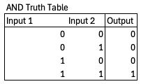
Every logic function will have a unique truth table, and for a given number of inputs and outputs there are only so many possible logic functions, so many possible truth tables. For instance, there are only four possible 1 input, 1 output functions.

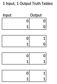
However, the space of possible logic functions gets very very large, very very quickly. For a function with n inputs and m outputs, the number of possible truth tables is (2^m)^(2^n). So if you have 2 inputs and 1 output, there are 2^4 = 16 possible functions (AND, NAND, OR, NOR, XOR, XNOR, and 10 others). If you have 3 inputs and 2 outputs, that rises to 4^8 = 65,536 possible logic functions. If you have 16 inputs and 9 outputs, like an 8-bit adder does, you have a mind-boggling 10^177554 possible logic functions. By comparison, the number of atoms in the universe is estimated to be on the order of 10^80, and the number of milliseconds since the big bang is on the order of 4x10^20. Fulfilling some goal from circuit space means finding one particular function in a gargantuan sea of possibilities.

The question is, how is the simulation able to navigate this enormous search space? Arthur touches on the answer — proceeding to complex goals by way of simpler goals — but he doesn’t really look deeply at the combinatorics in the paper, or how this navigation happens specifically.2

The emergence of circuits such as 8-bit adders seems not difficult. But consider the combinatorics. If a component has n inputs and m outputs there are (2^m)^(2^n) possible phenotypes, each of which could be realized in a practical way by a large number of different circuits. For example, an 8-bit adder is one of over 10^177,554 phenotypes with 16 inputs and 9 outputs. The likelihood of such a circuit being discovered by random combinations in 250,000 steps is negligible. Our experiment— or algorithm—arrives at complicated circuits by first satisfying simpler needs and using the results as building blocks to bootstrap its way to satisfy more complex ones.

Navigating large search spaces

In his 1962 paper “The Architecture of Complexity,” Nobel Prize-winning economist Herbert Simon describes two hypothetical watchmakers, Hora and Tempus. Each makes watches with 1000 parts in them, and assembles them one part at a time. Tempus’ watches are built in such a way that if the watchmaker gets interrupted — if he has to put down the watch to, say, answer the phone — the assembly falls apart, and he has to start all over. Hora’s watches, on the other hand, are made from stable subassemblies. Ten parts get put together to form a level 1 assembly, ten level 1 assemblies get put together to form a level 2 assembly, and 10 level 2 assemblies get put together to form the final watch. If Hora is interrupted in the middle of a subassembly, it falls to pieces just like Tempus’ watches, but once a subassembly is complete it’s stable; he can put it down and move on to the next assembly.

It’s easy to see that Tempus will make far fewer watches than Hora. If both have a 1% chance of getting interrupted each time they put in a part, Tempus only has a 0.99 ^ 1000 = 0.0043% chance of assembling a completed watch; the vast majority of the time, the entire watch falls to pieces before he can finish. But when Hora gets interrupted, he doesn’t have to start completely over, just from the last stable subassembly. The result is that Hora makes completed watches about 4,000 times faster than Tempus.

Simon uses this model to illustrate how complex biological systems might have evolved; if a biological system is some assemblage of chemicals, it’s much more likely for those chemicals to come together by chance if some small subset of them can form a stable subassembly. But we can also use the Tempus/Hora model to describe the technological evolution being simulated in Arthur’s paper.

Consider a technology as some particular arrangement of 1,000 different parts, such as the NAND gates that are the basic building blocks of Arthur’s logic circuits. If you can find the proper arrangement of parts, you can build a working technology. Assume we try to build a technology by adding one part at a time, like Tempus and Hora build their watches, until all 1000 parts have been added. In this version, instead of having some small probability of being interrupted and needing to start over, we have a small probability (say 1%) of correctly guessing the next component. This mirrors Arthur’s simulation, where we had a small probability of randomly connecting a component correctly to fulfill some goal. Only by properly guessing the arrangement of each part, in order, can we create a working technology.

In Simon’s original model, assembling a watch was like flipping 1000 biased coins in a row. Each coin had a 99% chance of coming up heads, and only when 1000 heads were flipped was a watch successfully assembled. Our modified model is like flipping 1000 biased coins which have only a 1% chance of coming up heads. Creating a technology via the “Tempus” method is like flipping 1000 coins in a row and hoping for heads each time. The probability of producing a working technology is 0.01^1000, essentially zero. But if we create a technology via the “Hora” method of building it out of stable subassemblies, the combinatorics become much less punishing. Now instead of needing to flip 1000 heads in a row, we only need to flip 10 in a row. 10 successful coinflips — 10 parts successfully added — gives us a stable subassembly, letting us essentially “save our place.” Flipping a tails doesn’t send us all the way back to zero, just to the last stable subassembly. The odds are still low — for each subassembly, you only have a 0.01^10 chance of getting it right — but it’s enormously higher than the Tempus design. You’re much more likely to stumble across a working technology if that technology is composed of simpler stable components, and you can determine whether the individual components are correct.

Arthur’s circuit simulation is able to find complex technologies because it works like Hora, not Tempus: complex circuits are built up from simpler technologies, the way Hora’s watches are built from stable subassemblies. Going from nothing to an 8-bit adder is like Tempus trying to build an entire and very complex watch by getting every step perfect. Much easier to be like Hora, and be the one that only needs to get the next few steps to a stable subassembly correct: adding a few components to a 6-bit adder to get a 7-bit adder, then adding a few to that one to get an 8-bit adder, and so on.

We can illustrate this more clearly with a modified version of Arthur’s circuit search. In this version, rather than trying to fulfill a huge collection of goals, we’re just trying to find the design for a specific 8-bit adder made from 68 NAND gates. Rather than build this up from simpler sub-components (7-bit adders, 6-bit adders, full adders), in this simulation we simply go NAND gate by NAND gate. Each iteration we add a NAND gate, and randomly wire it to our existing set of NAND gates. If we get the wiring correct, we keep it, and go on to try adding the next gate. If it’s incorrect, we discard it and try again.

We can think of this as a sort of modular construction, akin to building a complex circuit up from simpler circuits; at each level, we’re just combining two components, our existing subassembly and one additional NAND gate. This loses verisimilitude, since each subassembly no longer implements some particular functionality (we essentially just dictate that the simulation knows when it stumbles upon the correct gate wiring). But we don’t lose that much: it is, notably, possible to build an 8-bit adder with a hierarchy that requires just two components at almost every level (a few steps require three components). And this simpler simulation has the benefit of making it very easy to calculate the combinatorics at each step.

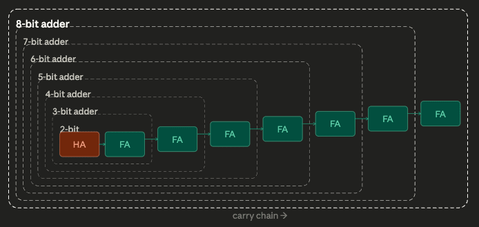Hierarchical 8-bit adder. FA is a full-adder (which adds 3 input values together), HA is a half-adder which adds 2 input values together). Full decomposition down to NAND gates not shown.

68 NAND gates can create around 2^852 possible wiring arrangements with 16 inputs and 9 outputs. This is much less than the 10^177,554 possibile 16 input and 9 output functions, but it’s still an outrageously enormous number. If we tried to find the right wiring arrangement by random guessing all 68 gates at once, we’d never succeed: even if every atom in the universe was a computer, each one trying a trillion guesses a second, we’d still be guessing for about 10,000,000,000,000…(140 more zeroes)..000 years.

But by going gate-by-gate, the correct arrangement can be found in 453,000 iterations, on average. Each time we add a gate, there’s only a few thousand possible ways that it can be connected, so after a few thousand iterations we guess it correctly, lock the answer in, and move on to the next gate. By determining whether each step is correct, instead of trying to guess the complete answer all at once, the search becomes feasible.

This is why Arthur’s original simulation couldn’t fulfill complex needs without fulfilling simpler needs first: if you try to take too many steps at once, the combinatorics become too punishing, and it becomes almost impossible to find the correct answer by random guessing. In our 68 NAND gate search, finding an 8-bit adder is relatively easy if we go one gate at a time, but if we change that to two gates at a time (randomly adding one gate, then another gate, then checking to see if we’re correct), the expected number of iterations rises from 453,000 to 1.75 billion: if the probability of guessing one gate correctly is 1/1,000, the probability of guessing two gates is 1/1,000,000. If we try to guess three gates at a time (1 in a billion odds of guessing correctly), the number of expected iterations to guess all 68 gates correctly rises to ~9.3 trillion.

The explosive combinatorics gives us a better understanding of some of the results that come out of Arthur’s simulation. For instance, Arthur notes that in each iteration the simulation combines up to twelve components, then checks to see if a working circuit has been found. But Arthur notes that you can vary the maximum value and it doesn’t impact the results of the simulation much, stating of the various simulation settings that “[e]xtensive experiments with different settings have shown that our results are not particularly sensitive to the choice of these parameters.” Indeed, if we re-run the simulation and only allow it to try a maximum of 4 components at once, it works basically just as well as with 12 components. The more random components you combine together, the more the combinatorial possibilities explode, and the lower the chance of finding something useful. The probabilities of finding a useful circuit amongst the various possibilities becomes so immensely low with larger numbers of components that you don’t lose much by not bothering with them at all. Similarly, this also explains another result in the paper, that it’s easier to find complex goals if you specify only a narrower subset of simpler goals related to them. Arthur notes that a complex 8-bit adder is found much more quickly if you only give the simulation a few goals related to building adders. With fewer goals specified, the pool of possible technology components will remain smaller, the number of possible random combinations becomes fewer, and the easier it becomes to find the complex goals.

In essence, using simpler components as stepping stones to more complex ones is a kind of hill-climbing. The simulation looks in various directions (possible combinations of building blocks), until it finds one that’s higher up the hill (finds a circuit that meets some simple goal), restarts the search at the new, higher point on the hill, until it reaches a peak (satisfies a complex goal). The simulation is able to satisfy complex goals because it specified a series of simpler ones that provide a path up the hill to the complex goals. Arthur notes that “[t]he algorithm works best in spaces where needs are ordered (achievable by repetitive pattern), so that complexity can bootstrap itself by exploiting regularities in constructing complicated objects from simpler ones.”

Trying to go to complex circuits directly, then, is akin to just testing random locations in the landscape and seeing if they’re a high point: this is obviously much worse than following the slope of the landscape to find the high points.

Technological search and information

We can sharpen these ideas even further by bringing in some concepts from information theory. Information theory was invented by Claude Shannon at Bell Labs in the late 1940s, and it provides a framework for quantifying your uncertainty, and how much a given event reduces that uncertainty.

I find the easiest way to understand information theory is with binary numbers. The normal math we use day to day uses base 10 numbers. When we count upward from zero, we go from 0 to 9, then reset the first digit to 0 and increment the next digit: 10. With binary, or base 2, we increment the next digit after we get to 1. So 1 in base 10 is 1 in binary, but 2 is 10, 3 is 11, 4 is 100, and so on.

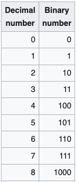Decimal (base 10) and binary (base 2) numbers.

In binary, each binary digit, or bit, doubles the potential size of the number we can represent. So with two digits, we can define 4 possible values (0, 1, 2, and 3 in base 10). With 3 digits, that doubles to 8 possible values (getting us from 0 through 7), with 4 digits that doubles again to 16 possible values, and so on. A 16 bit binary number can represent 2^16 = 65,536 possible values, which is why in computer programming the largest value that a 16 bit integer can represent is 65,535.

Say you have a string of bits, but don’t know whether they’re ones or zeroes. Because each bit doubles the number of possible values that can be represented, each unknown bit you fill in reduces the number of possible values by half. If you have 3 binary digits, there are 8 possible numbers that could be represented. Each time you learn what one of the bits is, you reduce the number of possible values by half.

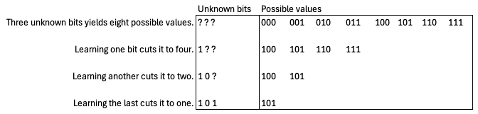
With information theory, we generalize this concept somewhat. In information theory one bit of information reduces the space of possibilities by 50%; in other words, each bit reduces our uncertainty by half. Say you’re like me, and you often lose your phone in your jacket pockets. If you’re wearing a coat with 2 pockets and you know the phone is in one of them, specifying the location of your phone, narrowing it down from 2 possibilities to 1, takes one bit of information. If you’re wearing a coat with 4 pockets, you now need 2 bits of information: 1 bit to tell you whether it’s on the right or the left, and another bit to tell you whether it’s an upper or lower pocket. The first bit cuts the possibilities in half, leaving you with two possibilities, and the second bit cuts it in half again. If your jacket has 8 pockets, now you need 3 bits to specify its location, and so on. The more places that something could be, the more information it takes to specify its location.

Information theory is particularly useful for quantifying how much information we get from some particular outcome. Say someone flips a fair coin; how much information do I get when they reveal whether it was heads or tails? Well, before they reveal it, I knew it could be one of two options, heads or tails. Revealing it narrows the number of possibilities from two down to one. We’ve cut the number of possibilities in half, and thus gained 1 bit of information. More generally, the information provided by some outcome is equal to -log2(the probability of that outcome). So revealing how a fair coin was flipped gives us -log2(0.5) = 1 bit. If we’re dealt a single card from a deck face down, when we reveal that card we’ve reduced the number of possible cards from 52 down to 1, and gained -log2(1/52) = 5.7 bits of information.

For a repetitive process, we also want to know a related quantity: entropy. Entropy is determined by calculating the information received from each possible outcome, multiplying it by the probability of that outcome, then summing all those values together. It’s the expected quantity of information you’ll get by taking some particular action.

Say I’ve lost my phone in my jacket with eight pockets, and am looking for it by randomly trying pockets until I find it. A random guess has a 1/8 chance of successfully finding the phone, and a 7/8 chance of coming up empty. Guessing correctly will yield me -log2(1/8) = 3 bits of information, as expected: once I guess correctly, I know the phone’s location. But an incorrect guess will yield me only 0.19 bits of information: I already knew most of the pockets don’t have the phone, so failing to find the phone in one pocket doesn’t tell me much that I didn’t already know. The entropy of a guess is (1/8) * log2(1/8) + (7/8) * log2(7/8) = 0.54 bits. When I first check a pocket, I can expect to get a little more than half a bit of information. (If I rule out pockets that I’ve already checked, the expected amount of information I get will rise each time, though if you’re like me you might have to check the same pocket a few times before you find the phone.)

Because each bit of information we get cuts the number of possibilities remaining by 50%, it doesn’t take that much information to narrow down an enormously large search space. The 2^852 possible circuits that can be created by wiring up our 68 NAND gates requires only 852 bits — 852 times cutting the number of possibilities in half — to specify. (That’s approximately the same number of bits that it takes to specify each letter of this sentence.)

A key aspect of entropy is that we maximize how much information we get when each outcome is equally plausible. So the entropy of a fair coin, with a 50% chance of coming up heads, is 1 bit. But if the coin has a 90% chance of coming up heads, the entropy is now just 0.46 bits. If the coin has a 99% chance of coming up heads, the entropy falls to 0.08 bits. When one outcome is very likely, you learn much less on each attempt, because you mostly get the outcome you already knew was likely. This is why when playing the game “20 questions,” the most efficient strategy is to try and ask questions where the answer divides the number of possibilities in half. “Is it bigger than a breadbox?” is a good starting question because there are probably roughly similar numbers of items that are bigger and smaller than a breadbox. “Is it a 1997 Nissan Sentra?” is a bad starting question because most possibilities are not a 1997 Nissan Sentra, so we learn very little when the answer is “no.”

We can think of our 68 NAND gate search as flipping a series of very biased coins, each one with a ~ 1/(several thousand) probability of coming up heads (where “heads” is “guessing the right wiring combination for that particular NAND gate”). The entropy of this process — the expected amount of information that we get — is very low, around 0.003 bits per attempt. Each attempt we learn very little about the correct wiring diagram (“it wasn’t this arrangement, it wasn’t this arrangement either, or this one”) so we need a lot of attempts — around 453,000, on average — to accumulate the 852 bits needed to specify the correct wiring for our 8-bit adder.3

Trying to guess two gates at a time is like biasing the coin even further: now each one has a ~1/(several million) probability of coming up heads. We thus get vastly less information per attempt — less than 0.000001 bits per attempt on average — so it takes us many, many more attempts to accumulate the information needed.

A useful way of thinking about our 68 NAND gate search is that it’s like a huge, branching tree. At every step — every time we add a gate — there are thousands of branches, each one representing one possible way to wire up the gate. Each branch then splits into thousands more (representing all the possible ways of wiring up the next gate), which split into thousands more, which split into thousands more, until at the end we have 2^852 possible “leaves,” each one representing a unique way of wiring up all 68 gates. Trying to get all 68 gates right at once, and then checking to see whether or not you did, is like examining one single leaf, one path from the base of the tree all the way to the tip of a branch. Not only are you overwhelmingly likely to guess wrong, but you haven’t narrowed down your possibilities at all: all you know is that one single leaf wasn’t the right answer, leaving you with the rest of the 2^852 possible leaves to sift through.

Checking to see whether each gate we add is correct before we proceed to the next one, by contrast, massively narrows down the number of possibilities. Whenever we determine a gate isn’t in the right spot, it eliminates every possibility that branches off from that point. If there are 1000 possible ways to wire each gate, each time we guess correctly we’ve narrowed down the possibilities downstream of that choicepoint by 99.9%. Huge swaths of possibilities get eliminated at each correct guess, letting us converge on the correct answer much more quickly.

The same basic logic applies to Arthur’s simulation. (In fact, in another publication, Arthur uses a very similar metaphor, describing technological search as trying to find a working path up a mountain, which is full of various obstacles.) Building up complex functions without the aid of intermediate, simpler ones is like trying to find a single leaf on a tree the size of the universe. Building up to complex circuits gradually, using simpler components as building blocks, lets you screen off huge branches of the tree at once. Once you have a working 2-bit adder, every branch that has a non-working 2-bit adder in it gets screened off. Your iterations yield massively more information, and the search problem becomes tractable.

Conclusion

The logic of Arthur’s simulation, and our simpler simulation, also applies to creating new technologies more generally. Logic circuits are a useful model to explore, because they’re real technology that is very amenable to simulation (they have a well-defined, simple behavior), but technology in general can be thought of as a combination of simpler components or elements arranged in various ways to create more complex ones. As Arthur notes:

…in 1912 the amplifier circuit was constructed from the already existing triode vacuum tube in combination with other existing circuit components. The amplifier in turn made possible the oscillator (which could generate pure sine waves), and these with other components made possible the heterodyne mixer (which could shift signals’ frequencies). These two components in combination with other standard ones went on to make possible continuouswave radio transmitters and receivers. And these in conjunction with still other elements made possible radio broadcasting. In its collective sense, technology forms a network of elements in which novel elements are continually constructed from existing ones. Over time, this set bootstraps itself by combining simple elements to construct more complicated ones and by using few building-block elements to create many.

One takeaway from this paper, as Arthur notes and we explored more deeply, is that a hierarchical arrangement of components, where a complex technology is made of simpler components, which are in turn made from even simpler components, makes it much easier to create some new technology. But a more general takeaway is that successfully creating some new technology means getting new information as quickly as possible. Working from (or towards) a hierarchical, modular design for some technology, where each element has some specific job it must do, makes it easier to find new technologies in part because you learn vastly more from each attempt at building one of those subparts. Knowing whether some entire complex function works or not tells you much less than knowing which individual component is working right, and what specific functionality needs to be corrected to fix the problem.

1

In addition to Brian Arthur, some other folks who I think have done really good work on this are Bernard Carlson, Clay Christensen, Joel Mokyr, Hugh Aitken, Edward Constant, and various folks associated with the Trancik Lab. There’s also a few folks, such as Joan Bromberg and Lillian Hoddeson, who have produced multiple very good technological histories that I return to often.

2

Indeed, we find that if we just randomly combine dozens of NAND gates, we get a random truth table almost every time, and never solve even medium-complex functions with a few inputs and outputs.

3

Adding things up, you find that the search actually yields over 900 bits, rather than 852 bits. This is due to the information overhead of a sequential search: you end up getting “extra” information that you don’t need. In our 8-pocket jacket search, if we just guess randomly it will take us on average 8 tries to find the phone. 8 attempts * 0.54 bits per attempt yields 4.32 bits, more than the 3 bits we need to actually specify the phone’s location.

Super Sport SS18 Glider yacht, via DesignBoom.

Welcome to the reading list, a weekly roundup of news and links related to buildings, infrastructure and industrial technology. This week we look at plastic price jumps, crypto-backed mortgages, a proposed AI data center pause, US battery manufacturing, and more. Roughly 2/3rds of the reading list is paywalled, so for full access become a paid subscriber.

War in Iran

The disruption to oil and LNG supplies caused by the closure of the Strait of Hormuz is causing some countries to burn more coal. “India is burning more coal to meet higher summer demand. South Korea has lifted caps on electricity from coal. Indonesia is prioritizing using its domestic supply. Thailand, the Philippines and Vietnam are boosting coal-fired power.” [NPR]

And because petroleum is used to make plastic, the closure of the strait is also driving up plastic prices. Dow Chemical plans a 30 cents per pound increase in April, following a 10 centers per pound increase in March. [WSJ] Plastic prices are up nearly 40% since February. [Reuters]

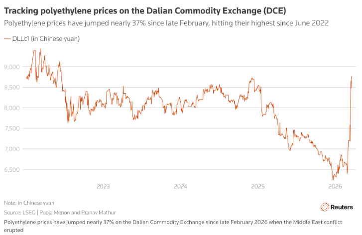
Petroleum is also used in the manufacture of pharmaceuticals, so the strait closure might affect the supply of generic medications. [CNBC] And last week I noted that production of helium (which is extracted as part of the natural gas drilling process) had also been disrupted, but I hadn’t clocked that liquified helium is used as a coolant for MRI machines. [X]

Another AWS data center in the mideast has apparently been damaged by an Iranian drone attack. [Al Jazeera]

To try and address rising gas prices, the EPA is temporarily waiving regulations on the sale of ethanol blended gas (which is restricted in certain locations at certain times of the year to reduce air pollution). [CNBC]

Iran has established a “safe shipping corridor” through the strait, allowing ships to pass for a $2m fee. [Lloyd’s List]

The closure of the strait seems to be good for Chinese battery manufacturers though: since the start of the war their stocks have spiked. “CATL’s China-traded shares have risen 19 per cent; Sungrow is up 19.4 per cent; and BYD, also the world’s top EV maker, has gained 21.9 per cent since the US-Israeli strikes were launched at the end of February.” [FT]

Housing

The New York Times on the ROAD to Housing Act, and the provision that would prevent the construction of build-to-rent single family homes. “Now, with the legislation back in the House awaiting a vote, critics are urging lawmakers to drop that build-to-rent restriction, arguing it would counter the intent of the bill, making it harder, not easier, to build homes when the country desperately needs them.” [NYT] Senator Elizabeth Warren is apparently unhappy about the resistance to these provisions of the bill, and is sending vaguely threatening letters to investors in multifamily apartments and manufactured homes. [Axios]

Another NYT article on the surprising success of some US malls. Apparently malls with higher-end, luxury tenants are doing fairly well. “There are roughly 900 malls in the United States, but only a small sliver are successful. The top 100 account for 50 percent of the entire sector’s value, according to Tibone, whereas the bottom 350 make up 10 percent. Revenue at class A malls is growing by 5 percent each year, and financing is easy to come by.” This is not totally surprising to me — malls in the Atlanta metro area seem crowded whenever I drive by or go in one, so I knew some must be succeeding — but it’s interesting to see that it seems to be specifically the high-end malls. [NYT]

Fannie Mae will now allow mortgages backed with cryptocurrency. “The mortgage company Better Home & Finance and the U.S. crypto exchange Coinbase Global unveiled a new mortgage product Thursday that allows home buyers to pledge their crypto holdings when getting a Fannie-backed mortgage, instead of selling the crypto to make a cash down payment.” What could go wrong. [WSJ]

Manufacturing

Elon Musk announces “Terafab” semiconductor fab to make chips for Tesla cars, Optimus, and space-based data centers. “We either build the Terafab or we don’t have the chips,” he said while on stage at an event in Austin. “We need the chips, so we’re going to build the Terafab.” [WSJ]

Read more

William Shockley, John Bardeen, and Walter Brattain, winners of the 1956 Nobel Prize for their work on the “transistor effect.” Via Wikipedia.

As we’ve noted more than a few times before, for most of the 20th century AT&T’s Bell Labs was the premier industrial research lab in the US. As part of its ongoing efforts to provide universal telephone service, Bell Labs generated numerous world-changing inventions, and accumulated more Nobel Prizes than any other industrial research lab.1 But the most important of its technical contributions proved to be useful far beyond the confines of the Bell System. Statistical process control, for instance, was invented by AT&T engineer Walter Shewhart to improve the manufacturing of AT&T’s electrical equipment at supplier company Western Electric. Since then, the methods have been successfully applied to all manner of manufacturing, from jet engines to semiconductors to container ships.

Interestingly, some of AT&T’s most important technological contributions — namely, the vacuum tube, the negative feedback amplifier, the transistor, and the laser — were (in whole or in part) the product of efforts to make new, better amplifiers for boosting electromagnetic signals. Amplifiers played a crucial role in the Bell System, making it possible to (among other things) connect telephones over long distances, but the value of these four amplifiers extended far beyond telephony. The vacuum tube became a crucial building block for electronics in the first half of the 20th century, used in everything from radio to television to the earliest computers. The negative feedback amplifier helped spawn the discipline of control theory, which is used today in the design of virtually every automated machine. The transistor is the foundation of modern digital computing and everything built on top of it. And the laser is used in everything from fiber-optic communications to industrial cutting machines to barcode scanners to printers.

It’s worth looking at why AT&T was so motivated to build better and better amplifiers, and why those efforts produced so many transformative inventions.

The vacuum tube

In 1876 Alexander Graham Bell placed the world’s first telephone call, summoning his assistant Thomas Watson from another room. By 1881, Bell’s company, the Bell Telephone Company (it wouldn’t become American Telephone and Telegraph, or AT&T, until 1899) had 100,000 customers. By the turn of the century AT&T was operating 1,300 telephone exchanges in the US, connecting over 800,000 customers with 2 million miles of wire.

The goal of the Bell System was “universal service” – to connect every telephone user with every other telephone user in the system. But by the early 20th century this quest was bumping up against technological limitations.

Telephones converted the sound of someone speaking to electrical signals, which were transmitted along wires until reaching a telephone on the other end, where they were converted back into sound. More specifically, in early telephones the sound from someone speaking would compress and decompress a chamber full of carbon granules, which would alter their electrical resistance, changing how much current flowed through them. At the other end, the electrical current would flow through an electromagnet, which pulled on a thin iron diaphragm; fluctuations in the electrical current would change the motion of the diaphragm, reproducing the speech.

But the farther electrical signals travelled, the more they would be attenuated. Resistance from the wire carrying them would convert some of the electrical energy into heat, and electrical current could “leak” between adjacent telephone wires. As the electrical signals got weaker and weaker, the sound would be less and less intelligible when reproduced, until it couldn’t be heard at all. If AT&T wanted to provide universal service, it would need a way to maintain the strength of the electrical signal as it traveled over long distances.

AT&T was able to partly resolve this problem using the loading coil, an invention of electrical engineer Michael Pupin. (Lines which had loading coils added to them were sometimes described as being “Pupinized.”) The loading coil added inductance (a tendency to resist changes in current) to telephone lines, which reduced signal attenuation. As a result, the loading coil roughly doubled the effective distance limit of telephone calls, from around 1000-1200 miles to closer to 2000 miles. But the loading coil merely reduced signal attenuation; the signal was still decaying as it traveled along the lines, just more slowly. Without some way of actually amplifying the telephone signals, the maximum distance for a telephone line was enough to connect New York to Denver, but not enough to reach the West Coast from New York and connect the entire country.

AT&T experimented with various mechanical amplifiers, which converted the electrical signals into mechanical movements and then back to electrical signals, but these were found to greatly distort the signal, and were not widely used. What was needed was an electronic amplifier, which could amplify the electrical signals directly, without the lossy and distorting effects of mechanical translation. In 1911, AT&T formed a special research branch to tackle the problem of long-distance transmission, and hired the young physicist Harold Arnold (who would later become the first director of research at Bell Labs) to research possible amplifiers based on the “new physics” of electrons.

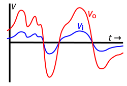Electronic amplification: the blue is the voltage of the input signal, which varies over time. The red is the amplified voltage of the output signal. The gain of this amplifier is three: output voltage is 3x input voltage. Similar amplification can be done for electrical current. Via Wikipedia.

At first, Arnold had little success. He looked at a variety of possible amplifying technologies, and experimented extensively with mercury discharge tubes (which initially seemed promising), but nothing appeared to fit AT&T’s requirements. But in 1912, Arnold learned of a new, promising amplifier known as the audion, which had been brought to AT&T by American inventor Lee de Forest. De Forest’s audion was, in turn, based on an invention of the British physicist Ambrose Fleming, known as the “Fleming valve.” Fleming was inspired by extensive experimentation with what was known as the “Edison Effect:” the observation that in an incandescent bulb, electric current would flow from the heated filament to a nearby metal plate. Fleming used this effect to create a diode, a device which lets electric current flow in one direction but not another. De Forest modified Fleming’s valve by adding a third element, a metallic grid, between the filament and the plate. By varying the voltage at the metallic grid, De Forest eventually discovered he could control the flow of electrical current from the filament to the plate. This allowed the device to act as an amplifier: a small change in the voltage could create a much larger change in the current flowing from the filament to the plate.

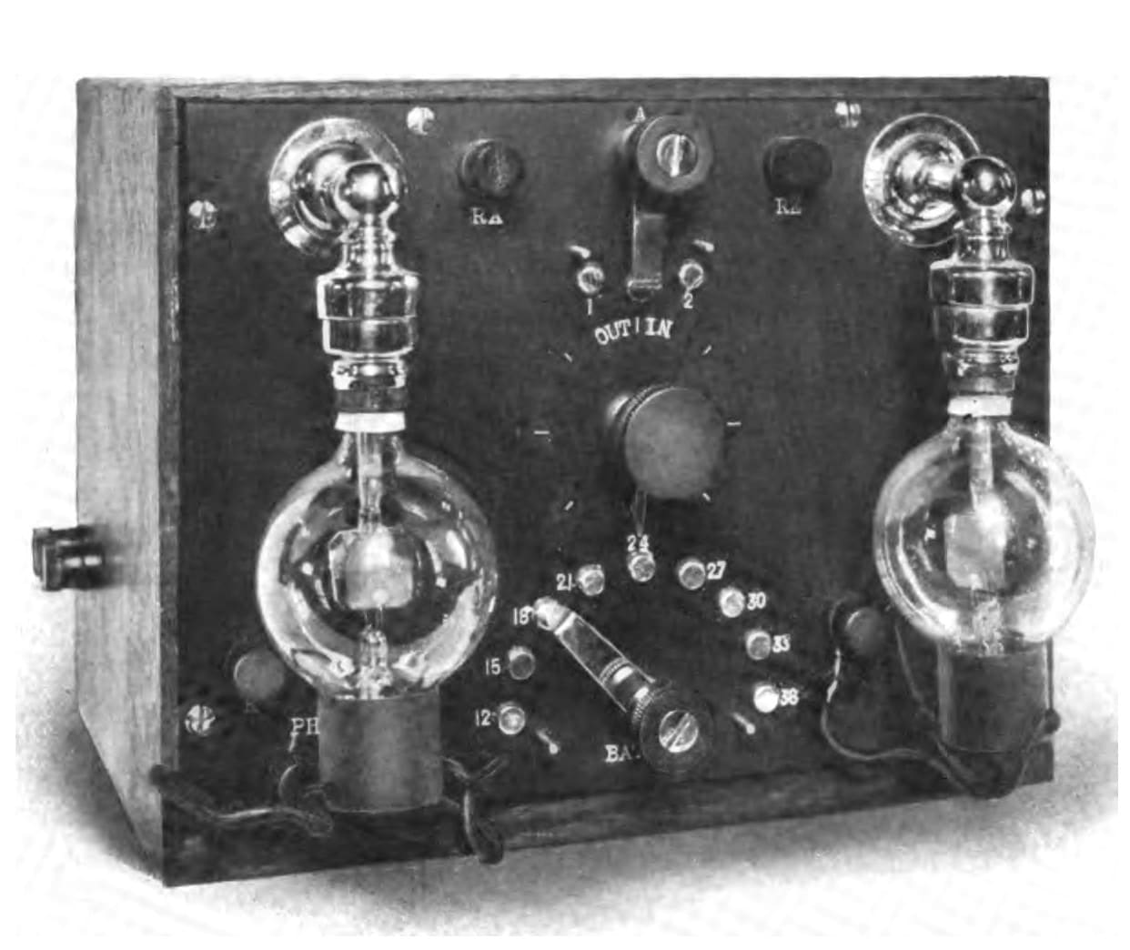A radio receiver built with audions, via Wikipedia.

De Forest’s audion had uneven performance — notably, it couldn’t handle the level of energy needed for a telephone line. Moreover, it was clear that De Forest did not quite understand how the device worked. But Arnold, well-versed in the physics of electrons, recognized its potential, and realized that, with modifications, its various limitations could be overcome. Via “The Continuous Wave,” a history of early radio:

Arnold knew exactly what to do about the audion’s limitations. “I suggested that we make the thing larger, increase the size of the plate with the corresponding increases in the size of the grid but particularly at that time I suggested that we were not getting enough electrons from the filament.” What he wanted to do, in fact, was convert the de Forest audion into a different kind of device. He wanted a much higher vacuum in the tube, with residual gas eliminated to the greatest possible extent; and he knew the newly invented Gaede molecular vacuum pump made that possible. He wanted more electron emission from the filament without an increase in filament voltage; and he knew Wehnelt’s new oxide-coated filaments would do that.

After paying $50,000 (roughly $1.6 million in 2026 dollars) for the rights to the audion, Arnold and others at AT&T spent the next year turning it into a practical electronic amplifier: the triode vacuum tube. By June 1914, vacuum tube amplifiers were being installed on a transcontinental telephone line connecting New York and San Francisco, and in January of 1915 the transcontinental line was inaugurated at the Panama-Pacific International Exposition with a call between Alexander Graham Bell in New York and Thomas Watson in San Francisco. By the late 1920s, AT&T was using over 100,000 vacuum tubes in its telephone system, and triodes and their descendents (four-element tetrodes, five-element pentodes) would go on to be used in all manner of electronic devices, from radios to TVs to the first digital computers.

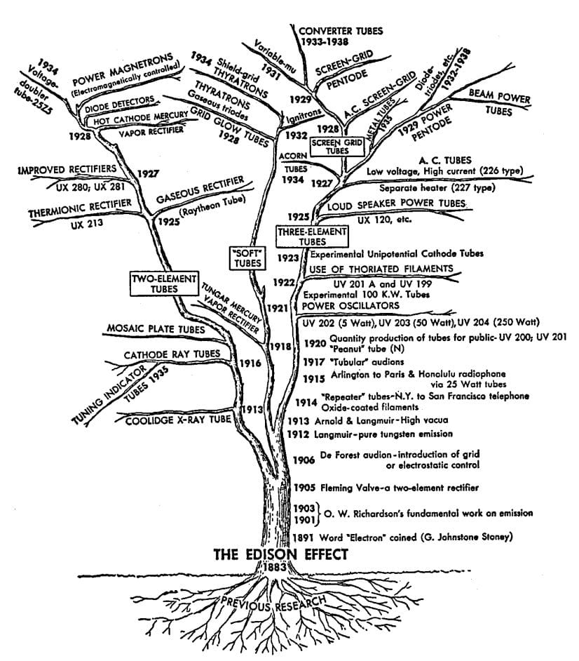Via Hong 2001.

The vacuum tube, with its ability to amplify electronic signals, represented a sea change in how AT&T engineers thought about telephone service. Prior to the electronic amplifier, a telephone call was essentially a single diminishing stream of electromagnetic energy. The range of that energy could be extended farther and farther from the speaker at the steep cost of its fidelity. The amplifier made it possible to consider a telephone call as a stream of information, as a signal that was distinct from the medium that carried it. It could be ably renewed, translated, modified in new and exciting ways. As historian David Mindell notes:

…a working amplifier could renew the signal at any point, and hence maintain it through complicated manipulations, making possible long strings of filters, modulators, and transmission lines. Electricity in the wires became merely a carrier of messages, not a source of power, and hence opened the door to new ways of thinking about communications…The message was no longer the medium, now it was a signal that could be understood and manipulated on its own terms, independent of its physical embodiment.

The negative feedback amplifier

Thanks to vacuum tube amplifiers, AT&T could finally fulfill its dream of universal telephone service, connecting telephones to each other anywhere in the continental US. But vacuum tubes were far from perfect amplifiers. The ideal amplifier has a linear relationship between the input and the output, effectively multiplying the input current or voltage by some value. If this relationship is non-linear, some inputs will be multiplied more than others, and the signal will become distorted. This distortion can garble speech, and — on a wire carrying multiple telephone calls — can create cross-talk, with speech from one telephone call being heard on another.

The vacuum tube was a superior amplifier to anything that preceded it, but it wasn’t a perfectly linear amplifier; its amplification curve formed more of an S-shape, under-amplifying low values and over-amplifying high ones. For a line carrying a single telephone call, the resulting distortion could be mitigated by restricting inputs to the linear portion of the curve, but as AT&T adopted carrier modulation — carrying multiple calls at different frequencies on a single line — distortion became more of a problem.

In 1921, Harold Black, a 23 year old electrical engineer, joined AT&T. He soon produced a report analyzing the future potential of a transcontinental telephone line carrying thousands of carrier-modulated conversations. At the time, carrier modulation was being used to carry at most three calls on a single line. Black’s analysis showed that such a line would require an amplifier with far less distortion than existing vacuum tubes,and Black began to work on developing an improved amplifier as a side project.

At first, Black simply tried to create vacuum tubes with less distortion, a project that many others at AT&T were also working on. The efforts of Black and others produced higher-quality vacuum tubes, but nothing Black tried reduced the distortion to the degree he was aiming for.

After two years of failure, Black decided to pivot; rather than trying again and again to build a perfectly linear amplifier, he would accept that any amplifier he made might be imperfect, and instead find a way to remove the distortion that it introduced.

Black first tried to do this by subtracting the input signal from the amplifier’s output, leaving behind just the distortion, and then amplifying that distortion and subtracting that from the output signal. This method — the “feedforward amplifier” — worked, but not well. It required having two amplifiers (one for the original signal, and one for the distortion) that needed to have very precisely matched amplification characteristics, and maintaining that alignment over a wide range of frequencies and for a long period of time proved difficult. As Black noted later:

For example, every hour on the hour —24 hours a day —somebody had to adjust the filament current to its correct value. In doing this, they were permitting plus or minus 1/2-to-l dB variation in amplifier gain, whereas, for my purpose, the gain had to be absolutely perfect. In addition, every six hours it became necessary to adjust the B battery voltage, because the amplifier gain would be out of hand. There were other complications too, but these were enough! Nothing came of my efforts, however, because every circuit I devised turned out to be far too complex to be practical.

Black grappled with the problem over the next several years, until suddenly realizing the solution while taking the ferry to work one morning in 1927. An electromagnetic signal consisted of a wave, alternating back and forth between positive and negative voltage. If you took a fraction of the output from an amplifier, and subtracted that from the input signal before it got amplified — by modifying the input with negative feedback — you would cancel out the distortion. Because this would reduce the strength of the input signal, this would have the downside of greatly reducing the how much the signal would be amplified (known as the gain), but that was ok; the distortion would be reduced so much that you could get as much gain as you needed by stringing several such amplifiers together. And unlike Black’s feedforward amplifier, this negative feedback amplifier would be self-correcting: any unexpected change to the gain in the amplifier would become a change in the feedback signal, compensating for the change.

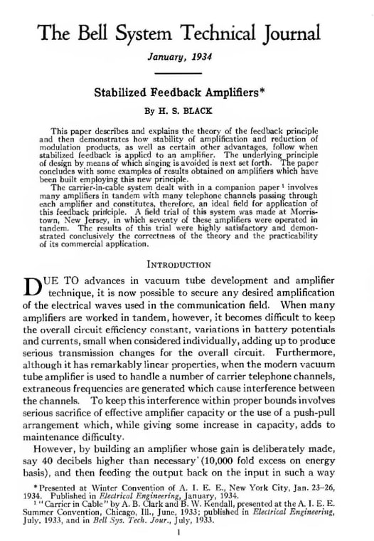Black’s first publication of the negative feedback amplifier, via Archive.org.

By the end of the year, Black had built a negative feedback amplifier that reduced distortion by a factor of 100,000. But Black had a difficult time convincing others of the merits of his invention. At the time feedback was largely considered undesirable by electrical engineers. Feedback could cause an amplifier to “sing” and start generating its own output, known as self-oscillation, overwhelming the input signal. (Think of the high-pitched sound that you get when placing a microphone next to a speaker.) Engineers went to significant efforts to prevent feedback-related problems.

At the time it was also believed that an amplifier with high levels of feedback would be fundamentally unstable. Opposition to Black’s amplifier was so severe that securing a US patent required “long drawn-out arguments with the patent office,” and the British patent office treated the invention the way they treated perpetual motion machines, demanding a working model. Harold Arnold, who had since become director of research at Bell Labs, “refused to accept a negative feedback amplifier, and directed Black to design conventional amplifiers instead.”

In practice, keeping the amplifier stable (avoiding self-oscillation) while also stringing together amplifiers in sequence proved to be a complex problem. These issues were resolved in part thanks to the help of two other Bell Labs researchers, Harry Nyquist and Henrik Bode. Nyquist and Bode studied the behavior of the negative feedback amplifier, and created mathematical tools for analyzing it and determining the conditions under which it would be stable.

Taken together, these efforts turned Black’s invention into a mainstay of electronics. Within 25 years, thanks to the work of Black, Nyquist, Bode, and others, the principle of negative feedback was “applied almost universally to amplifiers used for any purpose,” and it continues to be used in the design of modern amplifiers.

The effects of the Bell Labs work on negative feedback resonated far beyond amplification. A parallel tradition of feedback-based devices existed in mechanical engineering, in the design of things like governors and servomechanisms. During WWII, these two traditions began to merge into the modern discipline of control theory, which studies how to control a dynamic system using feedback. Feedback loops designed using control theory methods are the foundation of virtually every sort of automated system: aircraft autopilots, robotic arms, chemical plants, and the entire electrical grid all use feedback-based control loops, and the tools that Black, Nyquist, Bode, and others created to analyze the negative feedback amplifier are still used by control engineers around the world today.

The transistor

Even with negative feedback reducing their distortion, vacuum tubes were still far from ideal amplifiers. A vacuum tube is essentially a highly modified lightbulb, and has similar drawbacks as early lightbulbs: heating the filaments consumed a lot of power, and over time the tubes would burn out and need to be replaced. Mervin Kelly, a Bell Labs physicist who was promoted to director of research in 1936, wanted to replace the vacuum tube amplifiers and mechanical relays in the Bell System with solid-state devices, devices whose switching or amplification was done by way of electrons moving through a solid chunk of matter. Shortly after his promotion, Kelly began to hire physicists who were familiar with the then-novel physics of quantum mechanics, and could help better understand the behavior of solid matter. In 1938 Kelly created a group specifically devoted to solid-state research, and the team began working on building a solid-state amplifier using semiconductors: materials such as silicon, germanium, and copper oxide whose conductivity could be greatly varied. The group made progress — most notably, in 1939 Russell Ohl discovered that small amounts of impurities in silicon could drastically affect silicon’s conductivity when he accidentally created a photovoltaic cell in a silicon rod — but the work was soon disrupted by wartime priorities.

As the war progressed, Kelly recognized that wartime scientific and technological advances had the potential to upend the communications industry, and that if AT&T wanted to stay on top it needed to master the relevant sciences. He conceived of a new, major research program into solid-state physics that would be led by William Shockley, a physicist Bell Labs had hired in 1936 and who since 1938 had been researching solid-state devices.

During the war Shockley had worked on a variety of problems unrelated to semiconductors, including designing tactics for submarine warfare and training B-29 crews to use radar bombsights. But he also found time to work on a solid-state amplifier. In April of 1945, a few months before the end of the war, Shockley began to sketch out a device made from doped silicon (silicon with small amounts of impurities). Shockley hoped to use external electric fields to modify the conductivity of the silicon, amplifying the current flowing through it. His initial experiments, however, were met with failure.

A few months later, Kelly reorganized the research program at Bell Labs, creating a new, larger group wholly devoted to solid-state physics and led by Shockley. Among those who joined the new group were Walter Brattain, a physicist who had joined Bell Labs in 1929 and had previously studied copper oxide semiconductors, and John Bardeen, a new researcher from the Naval Ordnance Laboratory. Both were part of a subteam of the new solid-state physics group devoted specifically to the study of semiconductors.

Shortly after Bardeen joined, Shockley asked him to check Shockley’s calculations for the silicon amplifier in the hopes of learning why it hadn’t worked. Bardeen studied Shockley’s work, and eventually theorized that electrons might be getting “trapped” on the surface of the material, preventing the electric field from penetrating it and thus altering its conductivity. The semiconductor group began studying these “surface states,” and after nearly two years of experiments a breakthrough occurred.

Brattain had been studying surface states in silicon and germanium by shining light on the materials; if surface states existed, the light would knock away some electrons via the photovoltaic effect, “ripping holes in the semiconductor fabric.” Brattain discovered that not only was this electron disruption taking place, but that by varying the charge in an electrode above the surface of a piece of silicon, the strength of the photovoltaic effect could be varied significantly. The surface states themselves could be manipulated.

On November 21st, 1947 — a few days after Brattain’s discovery — Bardeen suggested using this ability to manipulate surface states to build an amplifier. They placed a sharp metal point onto the surface of a piece of doped silicon, and surrounded it with an electrolyte. By placing a small wire into the electrolyte and varying its voltage, they believed they could alter the conductivity of the silicon, and thus how much current flowed through it from the metal point.

The experiment worked: applying a voltage to the electrolyte boosted the current flowing through the metal point by about 10%. When Brattain rode home that night, he told the other members of his carpool that he’d “taken part in the most important experiment that I’d ever do in my life.”

Over the next several weeks, Bardeen and Brattain iterated on their new silicon amplifier. Initially its performance was poor, amplifying current only marginally, not amplifying voltage at all, and only functioning at very low electrical frequencies. But they eventually found that replacing the silicon with germanium allowed the device to amplify both current and voltage, and removing the electrolyte allowed it to amplify voltage over a wide range of frequencies.

By the middle of December, Bardeen and Brattain were ready to apply what they had learned. They fashioned a new device consisting of two thin pieces of gold foil attached to the surface of a piece of doped germanium, separated by only a 500th of an inch. They connected one wire to each of the pieces of gold foil, and a third to the piece of germanium. They reasoned that varying the current in one of the gold foil wires should amplify the current flowing through the other gold wire.

It worked: both current and voltage could be amplified across a wide range of frequencies using the device. Bardeen and Brattain had fashioned a solid-state amplifier.

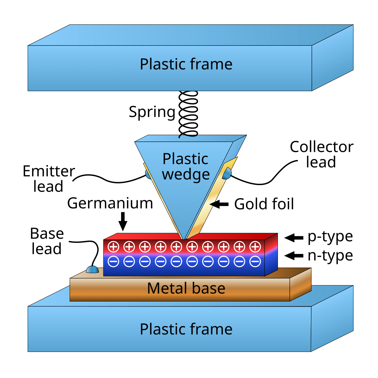Point contact transistor, via Wikipedia.

By early 1948, Bell Labs had fabricated nearly a hundred copies of Bardeen and Brattain’s amplifier (which would soon be named the transistor), and was testing how it could be used in various electronic devices. By the end of May, Bell Labs engineers had built a transistor-based telephone repeater. At a June 30th press conference, Bell Labs announced the transistor to the world:

We have called it the Transistor, T-R-A-N-S-I-S-T-O-R, because it is a resistor or semiconductor device which can amplify electrical signals as they are transferred through it from input to output terminals. It is, if you will, the electrical equivalent of a vacuum tube amplifier. But there the similarity ceases. It has no vacuum, no filament, no glass tube. It is composed entirely of cold, solid substances.

The rest, of course, is history.

Bell Labs worked out how to make the transistor more reliable, and by 1949 was manufacturing them by the thousands. William Shockley, irritated at not having taken part in Bardeen and Brattain’s discovery, worked to design an alternative semiconductor amplifier, the junction transistor. Shockley’s junction transistor, first successfully fabricated by Bell Labs physicists Gordon Teal and Morgan Sparks in 1950, was far more reliable than the point-contact transistor, and it would go on to be the most widely-used transistor until the MOSFET appeared in the 1960s. In 1956 Shockley, Bardeen, and Brattain would share the Nobel Prize in physics for the discovery of the “transistor effect,” by which time Shockley had left Bell Labs to found his own semiconductor company, Shockley Semiconductor Lab. In 1957, eight disgruntled employees would leave Shockley’s company to found Fairchild Semiconductor. Departing Fairchild employees in turn went on to found their own semiconductor companies, and the so-called “Fairchildren” (which include Intel and AMD) became the foundation of Silicon Valley. The world would never be the same.

The laser

As Shockley, Bardeen and Brattain were experimenting with semiconductors in the 1940s, another Bell Labs physicist, Charles Townes, was studying microwaves. Since the invention of radio in the late 19th century, the technology had progressed by steadily marching up the electromagnetic spectrum, finding ways to use shorter and shorter wavelengths. There were a variety of reasons for this: shorter wavelengths carried more information, there were limits to how many users could occupy a particular part of the electromagnetic spectrum, antennas for shorter wavelengths could be smaller, and radars with shorter wavelengths could resolve more detail. The shortest wavelengths in use in the 1920s were tens of meters in length, but by WWII this had fallen to centimeters in length; these were known as microwaves. During the war, at the behest of the military, Townes designed microwave radars of increasingly short wavelengths. When Townes designed a radar with a 10 centimeter wavelength, he was then asked to build a 3 centimeter one; when he built that, he was asked for a 1.25 centimeter wavelength.

But the pressure to achieve smaller and smaller wavelengths was bumping up against technological limitations. Generating and amplifying smaller and smaller wavelengths required smaller and smaller components; by the time wavelengths reached the millimeter range, the components to generate the signals became so small that manufacturing them, and putting enough power through them, became impractical. What was needed was a new way to generate and amplify radio signals that didn’t require fabricating microscopic components.

In 1948 Townes left Bell Labs for Columbia University, where he pursued research related to microwave spectroscopy. Townes hoped to use microwaves of increasingly small wavelengths, on the order of millimeters, to study the molecules and atomic nuclei. Because of his interest and expertise, and because shorter-wavelength radiation might prove valuable for radars or other military uses, Townes was asked by the Navy in 1950 to form an advisory group on millimeter wave radiation, so the Navy could keep abreast of any promising developments in the field. As there was not yet any good method of generating millimeter waves, most of the group’s efforts were focused on thinking of ways to generate them.

In April of 1951, on the morning of a day-long meeting of the committee, Townes awoke early and sat on a bench in a nearby park, and began to consider ways to generate millimeter wave radiation. Certain molecules, Townes knew, radiated energy at microwave wavelengths: perhaps instead of small electronic components, he could use molecules to generate the short millimeter waves he and everyone else were looking for?

The idea was not initially very promising. Molecules would certainly radiate after absorbing energy, but they would necessarily emit less energy than they absorbed — you couldn’t simply shine a light or send a signal through a collection of molecules, and get a stronger signal back. Heated molecules would radiate energy, but to generate microwaves they would need to be so hot that they would break apart into individual atoms.

Townes did know of one way to get a molecule to boost an electromagnetic signal: stimulated emission. Normally, when an atom or molecule is struck by a photon, its energy level will be raised. Later, when it falls back to its normal state, it will emit a photon. However, if it’s struck by a photon while it’s already in an elevated energy state, it will emit a second photon of the exact same frequency: one photon becomes two.

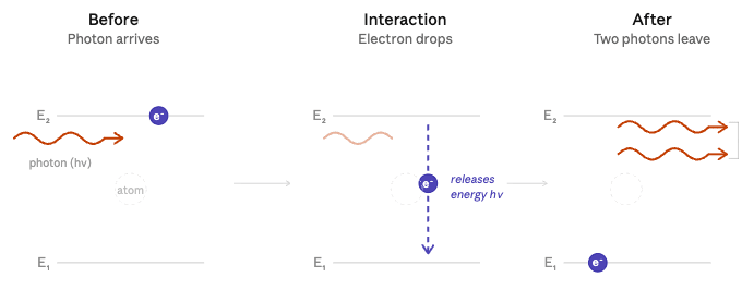Stimulated emission.

Most molecules are usually in low-energy states, not high energy states, which means that any amplification would quickly peter out as excess photons were absorbed. But Townes realized that if a collection of molecules could be coaxed so that most of them were in high energy states — known as a “population inversion” — a cascade of stimulated emission could take place. One photon striking a high energy molecule would become two; each of those could strike another high energy molecule, becoming four, then becoming eight, then becoming 16. A small amount of electromagnetic radiation could be amplified enormously. With enough molecules in an elevated state, Townes realized that in principle there would be “no limit to the amount of energy obtainable.”

Sitting in the park, Townes took an envelope from his pocket, and worked through how such a device might work. By feeding a stream of appropriately stimulated molecules into a resonator (a cavity that would reflect electromagnetic radiation of the appropriate wavelength), any electromagnetic radiation generated within the resonator would bounce back and forth, gaining energy each time it passed through the molecules as more and more photons were generated. The device would amplify any incoming signal as an electromagnetic wave passed through the population inversion molecules. And because the resonator would reflect the wave back and forth through the molecules (a form of feedback), it could also act as an oscillator — a generator of electromagnetic signals. Power would only be limited by how quickly molecules carried energy into the resonator.

A few months later Townes assigned Jim Gordon, one of his graduate students, the task of building the device, assisted by another graduate student, Herb Zeiger. Over the next several years Gordon worked diligently to realize the ambitious concept. Many physicists considered the idea unpromising: at one point, several years into the project, the current and former heads of Townes’s department, Isidor Rabi and Polykarp Kusch, exasperatedly stated to Townes that “you should stop the work you are doing. It isn’t going to work. You know it’s not going to work. We know it’s not going to work. You’re wasting money. Just stop!” But finally in 1954, a few months after Kusch insisted the device wouldn’t work, Gordon succeeded, demonstrating both amplification and oscillation in a collection of stimulated ammonia molecules. They called their device the maser, an acronym describing the device’s Microwave Amplification by Stimulated Emission of Radiation.

The maser, once developed, eventually proved to be “the world’s most sensitive radio amplifier,” an order of magnitude more sensitive than existing microwave amplifiers. Bell Labs, which hired Gordon in 1955, used masers to amplify the signals from its Echo and Telstar satellites launched in the early 1960s. The maser also found use in radio telescopes for astronomy. But the maser had drawbacks — most notably, it had to be cooled to a few degrees above absolute zero — and it was gradually relegated to increasingly niche uses as other low-noise amplifiers were developed.

The biggest impact of the maser was likely the invention that it inspired. In 1957, Charles Townes, still attuned to the problem of generating shorter and shorter electromagnetic waves, began considering how the maser might be adapted to such a task. Historically, radio had advanced into shorter wavelengths gradually, one step at a time. But Townes realized that with the maser it might be as easy, or perhaps even easier, to skip from microwave wavelengths (roughly 1 meter to 1 millimeter) all the way down to infrared or even optical wavelengths (roughly 0.000000380 to 0.000000750 meters). By this time, Townes had re-joined Bell Labs as a part-time consultant, and Townes and another Bell Labs physicist, Art Schawlow, worked through the physics of what they referred to as an “optical maser.” In 1958, they published a paper outlining the idea.

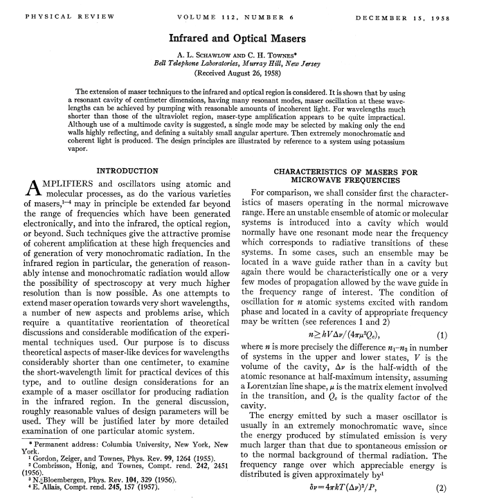Townes and Schawlow’s paper on optical masers, via American Physical Society.

After Townes and Schawlow’s paper was published, the race was on to build the optical maser, which soon began to be referred to as a laser, for Light Amplification by Stimulated Emission of Radiation). The first successful laser was built by Theodore Maiman at Hughes Aircraft in 1960 using a ruby crystal, but other successes quickly followed. It was soon discovered that a wide variety of materials could be made to “lase,” and before long there were lasers made from gasses, dye, glass, semiconductors, and more. In 1964, Townes would receive the Nobel Prize in physics for his work on the “maser-laser principle.”

While the laser could amplify signals that were passed into it, it proved much more useful as an oscillator, a generator of original signals. In 1959 Art Schawlow, believing that the laser would be more useful as an oscillator than an amplifier, jokingly suggested that it be renamed the LOSER. Unlike the maser, which was limited to niche uses, the laser proved to be useful for a wide variety of tasks. Within just two years of Maiman’s demonstration, a laser was used for eye surgery. By 1968, the US Air Force was dropping laser-guided bombs in combat. By 1971, Xerox PARC researchers built the first laser printer, and in 1974 the first laser-based barcode scanners were being installed. In 1980, the first commercial fiber optics lines using semiconductor lasers were made available. It’s the lasers ability to generate coherent light — light all of the same frequency, and in the same phase — that made it possible to continue to advance up the electromagnetic spectrum, and use optical wavelength electromagnetic radiation for communication.

Conclusion

Why did these various amplifiers, so many of them deriving from work at Bell Labs, end up being so valuable?

Partly it’s because an electronic amplifier is a very useful information processing device. An amplifier can amplify an electromagnetic signal, but it can also act as an electronic switch. And if the output of an amplifier is fed back into its input, an amplifier can also act as an oscillator: a generator of electromagnetic signals. Those are all useful information processing tasks, and each time a new, better amplifier was created, it extended the kinds of information processing that could be done. So these amplifiers were valuable because electronic information processing is valuable, and these amplifiers all greatly expanded the scope of information processing.

But a broader, somewhat more abstract reason is that many important technologies often act as amplifiers in one way or another. One of the most important inventions in biology, for instance, is the polymerase chain reaction, or PCR. PCR is essentially a DNA amplifier: it makes millions of copies of DNA sequences, making it far easier to study them and enabling things like the dramatic reduction in the price of genetic sequencing. The inventor of PCR, Kary Mullis, shared the 1993 Nobel Prize in Chemistry for his invention.

Examples of important amplifiers abound, because amplifiers themselves help produce abundance. Chemical catalysts, which can be thought of as amplifiers of chemical reactions, are used in everything from catalytic converters in cars to petroleum manufacturing. Simple machines like the lever or pulley amplify force, microscopes and telescopes amplify visual details. Industrial fermentation, nuclear reactors, the printing press, the Xerox machine, fractional reserve banking — all can be thought of as a type of amplifier.

So these four amplifiers were important in part because amplifiers in general are important. Amplifiers take something useful — an electromagnetic signal, a segment of DNA, a copy of a book — and make it possible to get a lot more of it, and technologies that do that are often particularly useful themselves.

1

For simplicity’s sake, I’m considering research done at AT&T before Bell Labs was formally incorporated as being done by Bell Labs.

Cargo ship Marine Angel navigating the Chicago River in 1953. Via History Calendar.

Welcome to the reading list, a weekly roundup of news and links related to buildings, infrastructure, and industrial technology. This week: damage to the Ras Laffan LNG facility, housing bubble risks, North Korea’s naval production, Bezos’ $100 billion for manufacturing automation, and more. Roughly 2/3rds of the reading list is paywalled, so for full access become a paid subscriber.

War in Iran

Ras Laffan, the world’s largest LNG facility in Qatar, was extensively damaged by an Iranian missile, and production has been completely shut down. The facility is responsible for something like 20% of the world’s supply of LNG, as well as for a third of global helium supply, which is used for semiconductor manufacturing. [Bloomberg] [CNBC]

Oil shipments from the UAE’s port of Fujairah have declined by two-thirds thanks to Iranian drone attacks. [Lloyds List]

To try and address rising oil prices following the closure of the Strait Hormuz, the Trump Administration has waived the Jones Act (which requires transportation between US ports to be done by US ships) for 60 days. [Reuters] It also invoked the Defense Production Act to order oil drilling to resume off the coast of California. [LA Times]

China tries to entice Taiwan to reunify by offering it energy security in the face of Middle East oil disruptions. [Reuters] And BYD dealerships are seeing a surge of interest in EVs. [Bloomberg]

Urbanist Richard Florida wonders if the war in Iran means the end of Dubai. Making your city a haven for the global elite means it’s relatively easy for them to relocate somewhere else if things turn south. “Dubai, which sits near the Strait of Hormuz, was supposed to be safe. Instead, it has been under attack by Iran since Feb. 28. More than 260 ballistic missiles and over 1,500 drones have been detected over the United Arab Emirates; most have been intercepted, but their percussive booms have become part of the city’s soundscape. The city that had spent decades billing itself as a sleek sanctuary — luxe, apolitical, income-tax-free, floating above and apart from the fractious region around it — was suddenly no longer insulated.” [NYT]

Housing

Swiss investment bank UBS has a report on which cities are at the highest risk of having a housing bubble, which they estimate by looking at trends in home prices, rents, and average incomes. Miami occupies the number 1 spot, followed by Tokyo and Zurich. [UBS]

Wired has an article about RealToken, which aims to “democratize access to real estate investment” by selling tokens representing shares of ownership in real estate properties. Apparently this has involved buying a bunch of dilapidated Detroit real estate and not maintaining it properly. “Last summer, the City of Detroit sued RealT and its founders, alleging “hundreds of blight violations.” Dorris’ property was one of many that city inspectors declared unfit for habitation. He told me that while his previous landlord wasn’t perfect, sometimes leaving Dorris to organize repairs, his building has deteriorated markedly since RealT entered the picture. The smoke detectors are missing, and the bathtub has no hot water, inspectors found. “The only way of washing is me standing over my sink,” says Dorris. “There are rats in the downstairs, there are squirrels in the upstairs.”” [Wired]

Marginal Revolution on how Denmark avoids the mortgage lock-in problem — where when interest rates rise, homeowners are reluctant to sell their home because their new one will have a higher interest rate mortgage. The Danish system has mortgages backed by a bond, which can be bought to pay off the mortgage. When interest rates rise, the price of the bond falls, incentivizing homeowners to purchase them. [Marginal Revolution]

Last Friday the Trump Administration released an executive order aimed at removing various regulatory barriers that add to the cost of building homes. [Whitehouse]

Read more