Donald G. Reinertsen's Blog

It seems obvious that the smart way to control of an epidemic is to prevent infected patients from triggering exponential chains of secondary infections. It also seems obvious that to do this we must first find infected patients. So, this is how we fight the war against Covid-19 today. We try to optimize the use of a single test to find a single infected patient. We focus on improving the accuracy, cost, and speed of this individual  test. And, we’ve done a great job; we test with a precision, efficiency, and speed that our predecessors could never dream of. Yet, there is a dark side. By focusing on the one test/one person problem, we have neglected another critical problem. This is what we might call the many tests/many people problem, a problem that is vitally important during an epidemic. What may not be obvious, is that the many people problem is very different from the single patient problem, and it has a very different solution.

Optimize a Single Test or A System of Many Tests?

Let’s use a simple analogy. We know that a chain is as strong as its weakest link. One way to make a strong chain is to separately test each individual link in the chain. We reason that if all the links are strong, then the chain will be strong. This frames the testing problem as a one link/one test problem.  A different way to view this problem is to see the chain as a system composed of many links. Viewed this way we would realize that we could attach 100 links together and test them in a single test. This allows us to use a single test to establish 100 links are good. The many links/many tests problem has a different solution than the one link/one test problem.

What does this have to do with Covid-19 testing? By now we have done about 20 Million Covid-19 tests worldwide. Most of the time, our test will establish that 1 patient is negative. Less frequently, it establishes that 1 patient is positive. What is certain is that we never identify more than one negative per test. What would happen if there was a way to identify as many as 10 to 30 negative patients in a single test? We would increase our testing capacity by a factor of 10 to 30. The 20 million tests we’ve already done could have done the work of 200 to 600 million individual tests.

The Magic of Sample Pooling/Block Testing

The method for producing more results per test is already in use. It is called sample pooling or block testing. It has been described in the Journal of American Medical Association. It has been reported on in the New York Times. It is used in Germany and Korea. It works by combining samples from 10 patients in a single batch and testing this batch in a single test. If the test is negative, which happens most of the time, it has identified that 10 patients are negative in a single test. If the test is positive, which happens less frequently, we need additional tests to determine how many patients were positive. The crucial difference is that we need much less individual testing. If a disease is only present in 1 percent of the population, 90 percent of the time a pool of ten tests will be negative, necessitating no additional tests. Sample pooling is perfectly suited for Covid-19 PCR testing because any dilution caused by combining 10 samples is trivial in the face of  the power of a PCR test to amplify the presence of DNA by a factor of a million.

What’s Stopping Us?

A key question is, why don’t we use this higher productivity approach to testing in America today? Quite simply, because our clinical laboratories are required to follow testing procedures mandated by the FDA and CDC. A clinical laboratory can lose its certification if it does not follow mandated procedures. Unfortunately, the current test prescribed by the CDC, , dated 3/30/2020, CDC 2019 Novel Coronavirus (2019-nCov) Real-Time RT-PCR Diagnostic Panel has no procedure for pooled samples, it only permits testing individual samples for individual patients. In other words, inefficient Covid testing is mandated by the US government.

We pay a high price for this inefficiency. Because we require 1 test per patient, we have a scarcity of tests. Because we have scarcity of tests, we focus these tests on people who already show Covid-19 symptoms. Since about 20 percent of Covid-19 infections are asymptomatic, this leaves thousands of untested people spreading Covid-19 through our communities. And, since scarce testing prevents us from locating the sources of infections in our community, we resort to brute force approaches like locking down our entire economy.

Even worse, in addition to forcing lockdowns, inefficient testing cripples our ability to reopen the economy. Reopening restarts the free movement of asymptomatic or pre-symptomatic people in a large pool of the uninfected people. This is only workable if we can find new infections quickly, trace their contacts, and quickly isolate them. While we can’t prevent all chains of infections, we can keep these chains short by shutting them down quickly. And, what does it take to find chain quickly? Frequent testing. Frequent testing is the key to preventing new waves of infection, and testing efficiency is what makes frequent testing cost-effective.

We Can Do Something

In fairness, the choice of the CDC and FDA to mandate inefficient testing is not motivated by malice. They are keenly aware of the danger of trying to fight an epidemic with unreliable testing and they are simply trying to do their job and promote public welfare. Test scarcity is simply an unintended and perhaps unexamined consequence of their choices. Now is a great time to change this and save lives.

Don Reinertsen

Testing capacity has been a major obstacle in the battle against Covid-19. Scarce capacity has led to the rationing of testing and to overloaded testing resources. Even today, it is not unusual to hear of 7 day waits for the results of a test that can be run in several hours. Such data suggests a process which is over 98% queue time, a clear symptom of overloads. This is a big problem.

The Solution Already Exists

Fortunately, there is an approach known as sample pooling that has the potential to increase testing capacity by at least an order of magnitude. And, it is already in use today. It was mentioned in a New York Times article of April 4, 2020 that discussed the unusual effectiveness of Germany’s Covid response. It stated:

“Medical staff, at particular risk of contracting and spreading the virus are regularly tested.  To streamline the procedure, some hospitals have started doing block tests, using the swabs of 10 employees, and following up with individual tests only if there is a positive result.”

On April 6, 2020, the JAMA website published a letter entitled “Sample Pooling as a Strategy to Detect Community Transmission of SARS-CoV-2. (2). It examined the effectiveness of processing 2888 specimens in 292 pooled samples. Both of these articles demonstrated the potential to improve existing capacity by close to 10x with sample pooling approaches.

What is Sample Pooling?

Sample pooling combines individual specimens into a pool or block. If a pool of ten specimens tests negative, this establishes that all ten specimens are negative using a single test. Only if the pool tests positive, is it necessary to allocate scarce capacity to individual tests. This approach exploits the high sensitivity of PCR tests. In fact, the CDC mentions sample pooling in its publications, but only as a strategy to lower testing cost, stating:

Available evidence indicates that pooling might be a cost-effective alternative to testing individual specimens with minimal if any loss of sensitivity or specificity. (3)

Sample pooling is particularly valuable in the early stages of an epidemic for two reasons. First, disease prevalence is still low, which means that a high percentage of pooled samples will test negative, making pooling highly efficient. Second, the early stages of an epidemic typically face the greatest capacity limitations, so improvements in capacity produce disproportionate benefits in finding and stopping disease propagation.

Sample Pooling and Information Theory

Interestingly, the mechanism of action behind sample pooling has strong parallels with ideas that have been exploited in software engineering for decades, ideas that might aid the use of this technique in medicine. In this article, I’d like to explore some insights from the engineering world that might be useful to the world of medicine.

The problem of finding infected patients in a large population, is similar to the problem of finding an individual item in a large pool of data. In software engineering, one approach for doing this is known as the binary search algorithm. For example, let’s say we want to find the number 12,345 in a sorted list of numbers. We would split the list in half and ask if the number was in the lower half or the upper half. We would then repeat this step on progressively smaller subsets until be found the answer. How much does this improve efficiency? For a list of 1,000,000 numbers a binary search can find the number with 20 probes rather the average of 500,000 probes required to search the same file sequentially. This difference has caught the attention of software engineers.

The high performance of the binary search comes from exploiting insights from the field of Information Theory. This field shows us how to generate the maximum possible information from each probe. By generating more information per probe, we need fewer tests are needed to complete our search.

From Information Theory, we know that a test with a binary answer, such as True/False  or Infected/Uninfected, will generate maximum information per test if the probability of passing (or failing) the test is 50 percent. Tests with low probability of failure are actually very inefficient at generating information. For example, if the probability of Covid positive outcome is 1 out of 1000, then the test generates surprisingly little information. If 1 out of 1000 patients is positive, then an individual Covid test, will identify 0.999 Covid negative patients per test. Let’s start with the numbers the appear in the JAMA letter, examine what was achieved, and ask if Information Theory would help us gain further improvements.

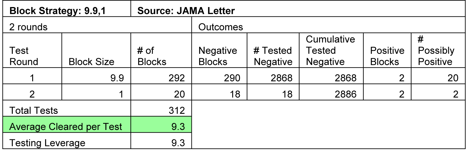
Round 1 Block Size 10 Gives 9.3x Improvement

If the subjects in the JAMA study were tested individually it would require 2,888 tests. By pooling the samples of 9 to 10 patients together, the probability that the pooled sample would test positive was increased. This raised the information generated by the test, thereby increasing the efficiency of the test. The same information was generated in fewer tests because there was more information per test. As a figure of merit for a testing strategy I have calculated the average number of negative patients produced per test, which I have labeled as Average Cleared per Test  in the following table. As the table indicates, the pooling strategy in the JAMA Letter was able generate 9.3 negative patients per test, compared to 0.999 negative patients per test with non-pooled tests. That raises productivity by 9.3x.

If we recognize this as an Information Theory problem, we can exploit ideas from this field to improve our solution. For example, maximum information is generated when a probe has a 50 percent success rate. In the JAMA study disease prevalence was 0.07 percent. At this level, there is only a 0.7 percent chance that that one of the 10 tests will be positive. This is nowhere close to the 50 percent rate required for optimum information generation.

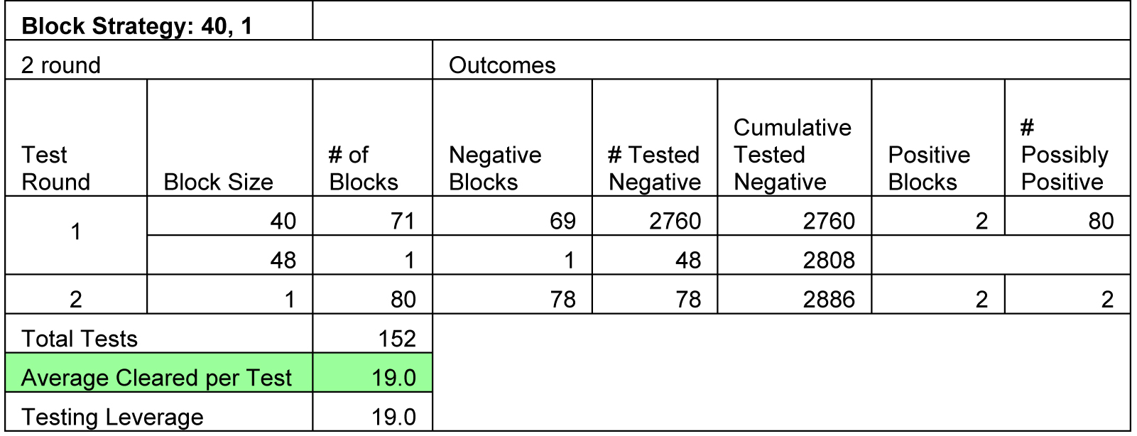
Raising Round 1 Block Size to 40 Gives 19x Improvement

So, let’s just look at what would happen if we raised our block size to 40 tests. As the table below indicates, we can generate 19 negative patients per test, more than doubling our productivity per test.  As Information Theory suggests, we can get more information out of a Round 1 test when we increase the likelihood of a positive test.

Note that to keep these calculations comparable I consistently use JAMA study numbers of 2888 patients with 2 positive cases.  I also make the conservative assumption that the two positive cases appear in different blocks. And, because 2888 total tests is not an integral number multiple of 40, I used 71 blocks of 40 tests and one block of 48 tests. The 80 potentially positive samples go into a second round of individual testing which finds 78 more negatives and 2 positive.

Using Three Rounds Give 41.8x Improvement

There is a disadvantage when large Round 1 block sizes are followed by a second round of individual tests. We are passing a large number of potentially positive tests into the intrinsically inefficient Round 2 of individual testing. For example, while a negative test on Round 1 block size of 500 could yield 500 negatives, a single positive within the block would require individual testing of all 500 samples within that block. Thus, we’ve created a need for a lot of low efficiency tests. We’d like to get the efficiency benefit that occurs when a pool tests negative, but we’d also like to reduce the penalty of using individual testing when we find a positive pool.

We can do this by using a more efficient strategy to search the positive pool. Instead of following Round 1 with individual testing, let’s insert an additional round of pooled testing before the round of individual testing. Why don’t we use a Round 1 block of 100, a Round 2 block of 10, and a final Round 3 of individual tests?  In effect, Round 2 will filter out additional negatives allowing Round 3 find the positives with fewer tests. In the example below Round 2 drops the number of samples that continue on to Round 3 from 200 to 20. This additional intermediate round allows us to generate 41.8  negative patients per test creating another doubling in productivity.

The additional intermediate round makes a big difference because it ensures that the pool of candidates reaching the inefficient final stage (1 test per patient) has a higher portion of positives. This, in turn, enables the final stage to generate more information per test. It works like the binary search algorithm which is extremely efficient is because it operates each round of testing near the theoretically optimum 50 percent failure rate.

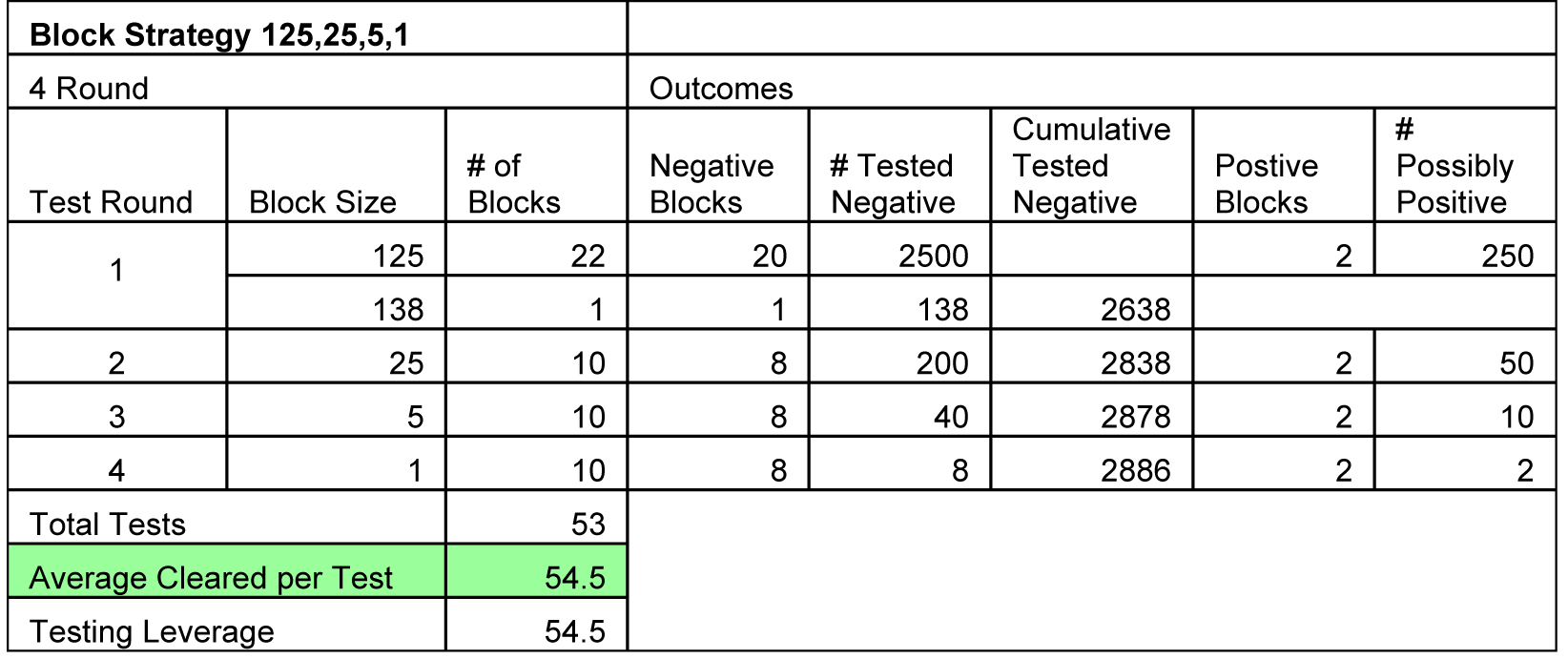
Moving to Four Rounds Gives 54.5x Improvement

Let’s look at the effect of adding an additional intermediate round which permits us to use a higher block size on the first round. The approach below uses 4 rounds of testing using blocks of  125, 25, 5, and 1.  Now we are up to 54.5 negative patients per test. This is a further improvement, although not a doubling.

Five Million Tests with Less Than One Negative per Test

Let’s look at the way we do Covid testing today in this context. As of today, we’ve done at least 5 million Covid-19 tests worldwide; almost all of these tests been done by inefficiently generating slightly less than 1 negative patient per test. Even worse, this inefficiency has occurred in the early stages of a pandemic when capacity was severely constrained, and when test productivity has the maximum possible impact.

If we generate information inefficiently our tests do less work. They give us fewer negative patients per test, larger backlogs, and massive queues. Yet, we vitally need test results to detect and control community transmission. We need them to find asymptomatic and presymptomatic spreaders. We need test results to trace contacts and isolate them before they start spreading. The queues we create with overloaded capacity delay testing and exponentially raise the number of secondary infections that we create while waiting for results. When we increase the efficiency with which we generate information we help almost every aspect of epidemic control.

The Crucial Role of Disease Prevalence

Sample pooling does not work equally well in all stages of an epidemic. Large blocks are efficient because they use a single test to find many negative cases. This works well when disease prevalence is low. However, if a single positive case shows up in the pool, the test will generate no negative cases. This means that as disease prevalence rises, sample pooling must use smaller and smaller block sizes. This in turn produces fewer and fewer negative tests per pool. In fact, at the point where 23 percent of the population is infected a Round 1 block size of 10 produces zero efficiency improvement over individual tests.

It is vital to recognize that the greatest benefits of sample pooling occur early in an epidemic. If we permit months of exponential spread before we use this powerful method, the epidemic may attain a prevalence at which sample pooling loses most of its benefits.

It’s Late but Not Too Late

Some opportunities to use Sample Pooling are gone, but future opportunities may be even greater. The explosion of Covid-19 spread has not yet reached highly vulnerable developing countries. Such countries have much more severe constraints in both testing capacity and the availability of people to perform the tests. They will most certainly face massive testing bottlenecks. This is still a perfect time to take what we have learned and use it to save lives.

Don Reinertsen

donreinertsen@gmail.com

310-373-5332

 

Additional Recommendations and Comments

1. Base the initial block size on the prevalence of the disease within the tested subpopulation. Large blocks only improve efficiency when disease prevalence is low. Once the disease has spread to more than 7% of a group a Round 1 block of 10 decreases in effectiveness. By the time 30 percent of group has a disease, a Round 1 block size of 10 will have a 97.2 percent chance of being positive, so it will almost never yield negative patients. Thus, sample pooling must be used early. This powerful tool loses its power when a disease becomes more prevalent.

2. Today’s multiple-round testing strategies tend to use pooled blocks in Round 1 to prefilter samples going into a final round of individual tests that have higher specificity and sensitivity. If we cascaded multiple levels of pooling prior to this final round of individual testing, these higher quality individual tests become more productive because they receive a flow of samples with more positives.

3. It is almost certain that larger blocks produce more sample dilution. Nevertheless,  it seems reasonable to expect that that nucleic acid amplification tests (NAAT) like qPCR tests, would be robust with respect to this dilution. This is a matter for true experts to decide. It seems likely that the intrinsic amplification of signals by 10^6 or more, would provide sufficient margin to tolerate the 100-fold dilution caused by pooling.

4. Regulatory risk could also be a huge obstacle. The CDC may view sample pooling primarily as a technique to reduce costs, rather than a technique to improve throughput. The FDA may view sample pooling as a modification of FDA-cleared procedures and therefore require special clearance under CLIA. There is quite likely a tension between the sincere desire of regulatory institutions to control risk, and the desire of clinicians to gain control over a rapidly growing epidemic. When infected cases double every 3 to 8 days, regulatory delays are clearly very costly. It would not be unreasonable to ask whether the damage caused by allowing thousands of untested people to contribute to the spread of a disease is more or less than the expected damage likely to come from a new method.  Judging pooled specimens as an unproven and therefore unusable technology may have great human costs.

References

1. Bernhold, K. (2020, April 4) A German Exception? Why the Country’s Coronavirus Death Rate is Low. The New York Times,  Retrieved from http://www.nytimes.com

-https://www.nytimes.com/2020/04/04/wo...

2. Hogan CA, Sahoo MK, Pinsky BA. Sample Pooling as a Strategy to Detect Community Transmission of SARS-CoV-2. JAMA. Published online April 06, 2020. doi:10.1001/jama.2020.5445

https://jamanetwork.com/journals/jama...

3. Centers for Disease Control and Prevention. Screening Tests To Detect Chlamydia trachomatis and Neisseria gonorrhoeae Infections — 2002. MMWR 2002; 51(No. RR-15): p.15.

https://www.cdc.gov/mmwr/pdf/rr/rr511...

Ward Cunningham introduced the “debt metaphor” to describe what can happen when some part of software work is postponed in order to get other parts out the door faster. He used this metaphor to highlight the idea that such postponement, while often a good choice, could have higher costs than people suspect. He likened the ongoing cost of postponed work to financial interest, and the eventual need to complete the work to the repayment of principal, observing that the interest charges could eventually become high enough to reduce the capacity to do other important work.

There is no question that technical debt is a useful concept. It easily communicates the danger of postponing important work. Even people who understand little about product development quickly grasp the idea that postponed work can overwhelm them, like a constantly growing balance on a high interest credit card.

Unfortunately, metaphors can cause us to treat a large class of situations as being essentially similar – even when they are not. In this case, we can avoid this trap by using the metaphor to identify the economic forces at work and using math to assess the balance of these forces.  Adding math to the metaphor is particularly useful in the case of technical debt because it allows us to think more clearly about a very wide range of situations.

Let’s begin by reviewing the economic characteristics of financial and technical debt.

Financial Debt

I’ll describe the simplest version of financial debt in which all principal is returned at the end of the loan period and recurring interest is paid regularly until the principal is returned. This is what most people have in mind when they use the debt metaphor.

When we incur a financial debt there are three economic consequences:

1. We receive access to an immediate benefit, the principal, which is of known magnitude and certain timing.

2. We incur an ongoing obligation to pay interest, which is an economic “rent” paid to the original owner of the principal. The timing and magnitude of these interest payments are also certain.

3. We undertake a future obligation to return 100 percent of the principal at a specific future time. Thus, the timing and magnitude of repayment is also certain.

Financial debt is not intrinsically evil.  It is economically sensible to incur financial debt when, by using the principal, we obtain risk-adjusted benefits that exceed the cost of the economic rent. For example, we might rationally borrow money to purchase a bicycle to avoid the recurring cost of paying daily taxi fares.

Technical Debt

If we consider technical debt to be analogous to financial debt, we could identify three similar economic consequences, although, as you will see, each one can take a wide range of forms:

1. We receive the benefit of postponing the expenditure of development effort. This benefit may include savings in both expenses and cycle time. The magnitude and timing of these benefits is uncertain.

2. We can incur an ongoing obligation to pay an economic “rent” on the deferred work. The magnitude and timing of this economic rent is also uncertain. It could range from positive to negative, and its timing can vary widely.

3. We incur a highly uncertain future obligation to repay the postponed development effort. Both the amount and timing of this future obligation is highly uncertain.

By analogy with financial debt, it is economically sensible to incur technical debt when the expected cost of the obligations incurred is lower than the benefits gained by deferring the work.  When we analyze the economics of technical debt we need to be particularly careful about two issues. First, we need to be sure we include the full economic costs. Second, we need to be sure we account for the uncertain nature of the costs. I’d like to illustrate how we can do this using three progressively more rigorous calculations.

First Iteration

Let’s take a simple case where we choose to introduce the product with technical debt rather than spending 2 months and $40,000 to design a debt-free product. In this case, assume we save $40,000 of development expense in year 1, pay extra support costs of $60,000 per year, and repay the deferred work in year 5 at twice the original effort for $80,000.  The table below shows these economics.

This is a bad economic proposition: our attempt to save $40,000 costs us $340,000. The answer looks compelling, but the calculation is faulty.

Second Iteration

Why? Because our first iteration ignored the cost of delaying the product launch by 2 months. We call the cost of delaying product introduction the Cost of Delay[1] (CoD), and it is quantifiable. So, I’ll add the delay costs for both the deferred and undeferred work on the lines highlighted in yellow.  In this case, we’ll assume our CoD is $250,000 per month and that the deferred work comprises 3 percent of the product value, and 3 percent of the delay cost. Therefore, the deferred work adds $90,000 per year of extra economic cost ($250,000 x 12 months x 3 percent), and the delivery of the undeferred work two months early saves us $485,000 ($250,000 x 2 months x 97 percent).

Note the striking difference in our answer when we consider delay costs. We see that we can defer the work for up to three years with no net economic cost. Yet, deferring the work for a full 5 years does not make economic sense. While this calculation is better, it still fails to recognize the uncertain nature of the costs.

Third Iteration

Now, let’s recognize that some of these costs are uncertain and adjust them for their likelihood. In this case, for simplicity, I’ve weighted all the costs associated with deferred work, highlighted in yellow, with a 50 percent probability of occurrence.  As a general rule we’d expect to have less confidence in costs associated with the deferred work than the undeferred work, and less confidence in costs at longer time horizons.

When we take into account the uncertain nature of these costs, we get a very different view of the problem. We can economically justify the full 5 years of deferral, although the cumulative benefit of this deferral decreases every year.  This answer is very different than our first calculation. Our view has shifted from an expected loss every year to an expected gain every year. This is the advantage of using math.

The point of these calculations is not to provide you with a new universal truth that can be substituted for thinking – it is to show you how a little math can illuminate the problem of technical debt.  Now, let’s discuss what factors you might consider in doing this analysis.

Some Tips on Doing Better Analysis

If you choose to incorporate some economic analysis into your decisions to postpone work, here are some tips that might help you:

Use an Economic Frame

Treat the decision to defer work as an economic choice rather than a philosophical one.  Weigh the likely economic benefits against likely costs.


When evaluating the economic benefits of deferring work, be sure to include both the work that is deferred and the work that is not. The economic impact on the undeferred work is often the dominant economic factor.


Since deferral affects development cycle time, it is crucial that we consider delay costs in our analysis. To assess this we must estimate the Cost of Delay for both deferred and undeferred work. Because 85 percent of developers do not quantify the Cost of Delay for their projects, they are poorly equipped to assess the real economics of deferring work.

Be Careful When Estimating Benefits Received

Recognize that the benefits from deferring work are uncertain. Be willing to weight them by their probability of occurrence. Will we really deliver the software any earlier if we postpone a work item? Will omitting the work really reduce our effort?


Focus on the net benefits.  Sometimes when we cripple a system by leaving out a key feature other activities will grow in cost and duration.  To assess net benefits we must look at both the deferred work and how this affects the rest of the project.


Be sure to include the value of feedback. Early feedback on the work that is released early can significantly reduce risk, and this risk reduction is worth money. In many cases, risk reduction will be a more important economic factor than the expense savings.

Estimate “Interest” with Care

Recognize that the recurring cost penalty associated with deferring work is uncertain. We are prone to overstate the benefits of our “debt-free” solution. This solution always appears to be far superior while it remains a figment of a programmer’s imagination, but sometimes, when instantiated into code, things are different.  Consequently, we should apply a discount factor on the savings that would arise from our “debt-free” solution.


Recognize the time dependency of the “rent” associated with deferred work. For example, we might target a 30 percent performance advantage over our competition, but early in life we may be able to generate customer preference with a 20 percent performance edge. Later, when competition has improved, our 20 percent edge may degrade to mere parity. Under such circumstances it can make economic sense to immediately harvest the benefits of our 20 percent advantage, and move to 30 percent before competitors reach parity. In such a case, the period during which we have a sufficient performance advantage can be viewed as “rent-free”. In such cases we can exploit the interest-free period and retire the debt before our interest charges start.


Recognize that at times there may never be any rent. If nobody actually cares about the feature, there will be no value created by delivering it early, and no cost when it is not yet available.


Recognize that at times the rent can be negative.  The feature we leave out may actually add more cost than benefit. In such cases, leaving it out makes us money.  For example, consider the choice of using a piece of open source software immediately, versus developing a superior solution by writing our own clever code.  The open-source code might create less utility for our customer, but it might also lower our support costs. When the savings in support exceed the lost utility we are paying a negative rent—deferring work reduces our ongoing costs instead of increasing them.

Evaluate Need to Repay Principal with Great Care

Don’t assume that it will cost the same to do work in the future as it does today. In most cases it will be cheaper to do it later because requirements will be better defined. However, in some important cases it can be very expensive to do the work later. When we create $1,000 of technical debt we might repay $2,000, $200, or absolutely nothing.


Don’t assume doing the work immediately will protect us from doing it again later. We may actually find that we are paying twice, and that our preemptive effort to do a “debt-free” design does not preempt very much at all.  If the cost to repay principal is the same whether we defer work or not, it should not enter into our calculations.

Pay Attention to the Larger System

Recognize how batch size reduction improves the economics of deferral . When we disaggregate the work into smaller chunks we dramatically increase the economic opportunity. If we defer 50 percent of work to permit 50 percent to be delivered early, then deferral costs will be high.  If we defer 1 percent of the work to permit 99 percent to be delivered earlier the economics are radically different.


Recognize how product architecture alters the combined economics of deferred and undeferred work. We can create “landing pads” for deferred work that minimize our future pain. Often a small burden on the work we are releasing early leads to big savings for the follow-on work. This is particularly true when we provide extra margin in a product architecture aligned with its likely growth vectors.


As mentioned earlier, recognize the feedback benefits of deferring work. Reductions in the scope of work permit us to deliver functionality faster. This gives us early feedback. Early feedback allows us to truncate unproductive paths more quickly. Such feedback can be exploited to alter the economics of subsequent decisions.


Treat the economics of deferred work as something we can control, not an immutable characteristic of the work.  The value of understanding our economics is that it helps us find the best places to intervene in our system.

Consider Calling It Deferred Work

When we refer to postponed work as technical debt this automatically biases us to assume that both ongoing and future costs are more certain than they really are. This, in turn, causes us to overestimate these costs, leading us to be overly cautious about deferring work. If it is your intention to bias the decision against postponement, this is clearly the best term to use. However, if you are trying to carefully weigh of pros and cons of postponing work, I’d recommend using a more neutral term like deferred work. In finance the concept of deferral is well understood. There are economic reasons for deferring revenues and expenses; managers are familiar with deferred assets and deferred liabilities. Calling it deferred work captures the economic essence of what we are doing without any positive or negative connotation.

Conclusion

To be perfectly clear, I am not suggesting that the debt metaphor never applies, only that it is less reliable in the domain of product development than some of its users think. There will be times when technical debt behaves exactly like financial debt and others times when the differences are enormous. Reasoning purely by metaphor may lead to bad economic choices – adding some math can lead to good ones.

In fact, there is another important advantage gained by enhancing your view of technical debt with a bit of economics: the people you are trying to influence care about the economic effects of their decisions. When you frame choices in economic terms you can communicate your ideas to them in their preferred language. Don’t underestimate how much effort and frustration this will save you.

Don Reinertsen

[1] Cost of Delay will be a new idea to some readers, but it is discussed in all of my books.

The post Technical Debt: Adding Math to the Metaphor appeared first on Reinertsen & Associates.

Nobody likes a fragile design; when you provide it with the tiniest excuse to fail, it will. Everybody likes robust systems. Robustness can be defined many ways, but I think of it as the ability perform as intended, in the presence of a wide range of both expected and unexpected conditions. Thus, a robust system is relatively imperturbable.

As engineers, how do we achieve this robustness? Two general approaches are passive and active robustness. Passive robustness uses design margin to reduce the magnitude and likelihood of the undesired response. Active robustness uses feedback loops to counteract the perturbation.

Consider the problem of preventing a sailboat from capsizing in unpredictable gusts of wind. One passive approach is to add ballast to lower the center of gravity. This will increase righting moments by increasing the distance between the center of buoyancy and the center of gravity. As a result, the boat will not heel over as easily. Unfortunately, this robustness comes at the expense of performance; since the boat is heavier, it will not sail as fast. Importantly, we pay the cost of passive robustness in both strong and light winds, when we need it, and when we don’t.

In contrast, active robustness uses feedback loops to respond to changes in the wind. For example, we might ease off our heading in the presence of a strong gust. We might have the crew hike out on the windward side of the boat to counterbalance the heel. An active approach allows us to expose more sail area and sail the boat faster in the presence of variable winds. We are safe because our feedback loops prevent dangerous conditions from developing. With active robustness we sacrifice less performance than we do with passive robustness, since our feedback loops only dampen response when this is necessary.

However, though active robustness is normally superior to passive robustness, it does have a dark side. The feedback loops can mask the progressive deterioration of performance and set us up for sudden and catastrophic failure. Ironically, the more effective our active feedback loops, the more vulnerable we are to such a catastrophic failure.

Let’s illustrate this phenomenon using the exquisitely well-designed feedback loops of the human body. The body uses many feedback systems to achieve robust performance in the presence of trauma. The medical term for this is homeostasis: maintaining a stable state. For example, when an accident victim bleeds severely they experience what is called hypovolemic shock. Their blood loss can prevent sufficient oxygenated blood from reaching vital organs such as the brain. This can reduce brain function, endangering survival. The body responds to this blood loss by activating feedback loops to maintain the flow of oxygenated blood the brain. Heart rate, breathing rate, and heart stroke volume increase; vasoconstriction decreases blood flow to non-critical organs. This stage of shock is called “compensated shock,” because the body successfully maintains blood pressure by compensating for the loss of blood volume.

But, what happens if the victim continues to lose blood? Eventually, the feedback loops have done everything they can to maintain blood pressure, and it is inadequate—the body transitions to “uncompensated shock”. In this stage it is unable to maintain blood flow to the brain, heart, and lungs; the availability of oxygenated blood drops rapidly; and sadly, you die. Uncompensated shock quickly leads to rapid, irreversible, and catastrophic deterioration.

During the initial stage of hypovolemic shock, the compensating mechanisms maintain blood pressure and prevent the most serious consequence of blood loss—reduced perfusion to the brain. System deterioration is occurring, but it does not appear as a drop in blood pressure. Let’s think of blood pressure a Key Performance Indicator (KPI), since it is. In fact, it is so important that our body’s feedback loops manage it very effectively. Unfortunately this effectiveness can mask the victim’s deteriorating physical condition. In fact, the more successful the feedback loop, the more it hides the real deterioration. The KPI does not tell us that system performance is deteriorating. Specifically, it does not tell us that we are losing our margin of safety, that is the size of a perturbation that the system can now cope with.

Of course, similar problems occur in product development. We can focus on the big three KPIs: performance, cost, and schedule and fail to pay attention to our safety margin. Suppose an overaggressive schedule causes the team to fall behind on their work. They compensate by heroically working longer hours, and no milestones are missed: performance, schedule, and cost are on track. Should we worry? Yes, we are losing our safety margin and our project is becoming riskier.

What should we do? Monitor the safety margin in your feedback loops in addition to your KPIs. In the case of compensated hypovolemic shock, even when blood pressure was not dropping, the signs of trouble were clearly present. Heart rate and respiration rate were up; vasoconstriction was making the skin pale and clammy. The signs of decreasing safety margin are always present, if you know what to look for. Do you think you have no worries because you haven’t missed a milestone? Check to see if your team’s average work week has increased from 50 hours to 100. If so, you are living on borrowed time.

There is also a psychological trap when we only focus on KPIs like schedule, cost, and performance in a system with effective feedback loops. We will see a project repeatedly absorb perturbations with no effect on our KPIs. This conditions us to incorrectly believe that similar future perturbations will be absorbed equally gracefully. If you don’t monitor the feedback loops you will be unable to see the real consequences of the absorbed perturbations.

What should you do? If you just want simple solutions, restrict yourself to passive robustness. If you need higher performance, use active robustness, but be fully aware of its risks. You can manage these risks if you know how your important feedback loops work. What compensation mechanism is maintaining the performance of your KPIs? How much capacity does your system have to compensate? How much of this capacity have you already consumed? You will be much less vulnerable when you know exactly what is standing between you and catastrophe.

Don Reinertsen

The post The Dark Side of Robustness appeared first on Reinertsen & Associates.

Some product developers observe that failures are almost always present on the path to economic success.  “Celebrate failures,” they say. Others argue that failures are irrelevant as long as we extract knowledge along the way. “Create knowledge,” they advise. Still others reason that, if our real goal is success, perhaps we should simply aim for success. “Prevent failures and do it right the first time,” they suggest. And others assert that we can move beyond the illusion of success and failure by learning from both. “Create learning,” they propose.  Unfortunately, by focusing on failure rates, or knowledge creation, or success rates, or even learning we miss the real issue in product development.

In product development, neither failure, nor success, nor knowledge creation, nor learning is intrinsically good. In product development our measure of “goodness” is economic: does the activity help us make money? In product development we create value by generating valuable information efficiently. Of course, it is true that success and failure affect the efficiency with which we generate information, but in a more complex way than you may realize. It is also true that learning and knowledge sometimes have economic value; but this value does not arise simply because learning and knowledge are intrinsically “good.” Creating information, resolving uncertainty, and generating new learning only improve economic outcomes when cost of creating this learning is less than its benefit.

In this note, I want to take a deeper look at how product development activities generate information of economic value. To begin, we need to be a little more precise on what we mean by information. The science of information is called information theory, and in information theory the word information has a very specific meaning. The information contained in a message is a measure of its ability to reduce uncertainty. If you learn that it snowed in Alaska in January this message contains close to zero information, because this event is almost certain. If you learned it snowed in Los Angeles in July this message contains a great deal of information because this event is very unlikely.

This relationship between information and uncertainty helps to quantify information. We quantify the information contained in an event that occurs with probability P as:

As we invest in product development, we generate information that resolves uncertainty. We will create economic value when the activities that generate information produce more benefit than cost. Since, our goal is to generate valuable information efficiently, we can decompose our problem into three issues:

How do we maximize the amount of information we generate?
How do we minimizing the cost of generating this information?
How do we maximize the value of the information we generate?

Let’s start with the first issue. We can maximize information generation when we have an optimum failure rate. Information theory allows us to determine what this optimum failure rate is. Say, we perform an experiment which may fail with probability Pf and succeed with probability Ps. The information generated by our experiment is a function of the relative frequency with which we receive the message of success or failure, and the amount of information we obtain if failure or success occurs. We can express this mathematically as:

We can use this equation to graph information generation as a function of failure rate.

Note that this graph maximizes at a 50 percent failure rate. This is the optimum failure rate for a binary test. Thus, when we are trying to generate information it is inefficient to have failure rates that are either too high, or too low. Celebrating failure is a bad idea, since it drives us towards the point of zero information generation on the right side of the curve. Likewise, minimizing failure rates drives us towards the point of zero information generation on the left side of the curve. So, we address the first issue by seeking an optimum failure rate.

But, this is only part of the problem. Remember, we generate information to create economic value, and we create economic value when the benefit of the created information exceeds the cost of creating it. So, let’s look at the second issue: how do we minimize the cost of generating information?

This is done best by exploiting the value of feedback, as I can illustrate with an analogy. Consider a lottery that paid a $200 prize if you pick the correct 2 digit number. If it costs $2 to play, then this lottery is a break-even game.  But, what would happen if I permitted you to buy the first digit for $1, gave you feedback, and then permitted you to decide whether you wanted to buy the second digit for an additional $1? The second game is quite different. It still requires the same amount of information (6.64 bits) to identify the correct two digit number, but it will cost you an average of $1.10 to obtain this information instead of $2.00. Why? You are buying in information in two batches (of 3.32 bits each). However, because you will pick the wrong first digit 90 percent of the time, you can avoid buying the second digit 90 percent of the time, saving an average of $0.90 each time you play the game.  (In the language of options, buying one digit at a time, with feedback, creates an embedded option worth $0.90.) Thus, we address the second issue by breaking the acquisition process into smaller batches and providing feedback after each batch. (Lean Start-up fans will recognize this technique.)

The third issue is to maximize the value of the information that we acquire. The most useful way to assess value is to ask the question, “What is the maximum amount of money a rational person would pay for the answer to this question?” For example, if one of two envelopes has a $100 bill in it, what should you pay to know which envelope it is in? Certainly no more than $50, the expected value of picking a random envelope with no information. Thus, to get the $100 envelope you should pay no more than $50 for the 1 bit of information it takes to answer the question. If the amount in the envelope is $10, you should not pay more than $5 to know which envelope the money is in. In both cases, it takes one bit of information, but the value of this bit is different.

So we address the third issue by asking questions of genuine economic significance, and making sure the answer is worth the cost of getting it. In reality, we do not have unlimited resources to create either learning or knowledge; we must expend these resources to generate information of real value.

My guess is that your common sense has already reliably guided you to address these three issues. For example, when you play the game of 20 questions, you instinctively begin with questions that split the answer space into two equally likely halves. You clearly understand the concept of optimum failure rate. When you decide to try a new wine you buy a single bottle before you buy a case. You clearly recognize that while small batches and intermediate feedback will not change the probability that you will pick a bad wine, they will reduce the amount of money that you will spend on bad wine.  And, when your encounter two technical paths that have virtually identical costs, you don’t invest testing dollars to determine which one is best. You clearly recognize that information is only worth the value it creates. If you do these things, you should have little risk of blindly celebrating failure, success, knowledge creation, or learning. If your common sense has not protected you from these traps, an excellent substitute is to use careful reasoning. It will get you to the same place, and sometimes even further.

Don Reinertsen

The post The Four Impostors: Success, Failure, Knowledge Creation, and Learning appeared first on Reinertsen & Associates.

In Lean Manufacturing one-piece flow is the state of perfection that we aspire to. Why? It unlocks many operational and economic benefits: faster cycle time, higher quality, and greater efficiency. The economically optimal batch size for a manufacturing process is an economic tradeoff, but it is a tradeoff that can be shifted to favor small batches. We’ve learned to make one-piece flow economically feasible by driving down transaction cost per batch. One-piece flow is unquestionably a sound objective for a manufacturing process.

But, is one-piece flow also a state of perfection for product development? In my experience, product developers actually have fewer constraints than manufacturing and this creates far greater opportunities for batch size reduction. In product development it is quite practical to decrease lot sizes below one item.

In manufacturing we handle physical objects, and physical objects can only be in one place at a time.* The shaft is either on the lathe or the grinder – it cannot be in both places at once. In product development we work on information, and information can be in two places at the same time. This creates opportunities that do not exist in manufacturing.

Let’s start with a simple example. In product development we often produce engineering drawings that prescribe many important characteristics of a manufactured part. If such drawings are viewed as physical objects, then the smallest quantity of information that can be transferred is one drawing. Engineering finishes its work and then transfers its work product to manufacturing.

The smartest product developers do not operate this way. Instead they recognize that the information on a drawing can be divided into much smaller batches. A drawing typically specifies many details about a part. In the limit, each individual detail can be transferred in a separate batch. A drawing with 100 dimensions might allow us to drop our batch size by another two orders of magnitude.

Of course, in practice we never go to this theoretical limit because we still must respect the economic tradeoff between holding cost and transaction cost. It rarely makes sense to transfer single dimensions because transaction cost dominates at very small batches and the value of receiving an isolated dimension is often quite small. So, while we routinely use batch sizes smaller than a complete drawing, I’ve never seen companies transfer one dimension at a time. Most often, we break the drawing up into multiple release levels, at times as many at 6 to 8, and freeze certain data elements at each release level.

But, let’s push a little harder on this. Is transferring one dimension at a time really our theoretical lower limit? No, and this is where it gets interesting. While a single dimension may appear to be the smallest atomic unit we can transfer, this is not the case when we are transferring information.

To explain this I need to clarify how engineers think about information. Engineers measure the amount of information contained in a message by the amount of uncertainty it resolves. If p is the probability of an event, then the information contained in knowing that event occurred is:

Information = – log2 (p)

 One bit of information is sufficient to identify which of two equally likely outcome has occurred. (When p = 50%, then I = 1.) Two bits is enough information to distinguish four equally likely outcomes. More probable outcomes have lower information content, and less probable ones have more information content. If I told you there was an 80 percent chance of rain tomorrow when it actually rains this outcome contains 0.32 bits of information. If it does not rain, which is less probable, more uncertainty is resolved and this outcome provides 2.32 bits of information. Notice that information can come in quantities smaller than one bit, and therein lies the opportunity. We do not have to treat an individual fact as the atomic unit that sets the lower limit on batch size. We can transfer information about a fact in multiple small batches as our confidence in this fact grows.

Perhaps an example would help. I was once working with a semiconductor company that was designing a specialized chip for the TV industry. Classic development practice would require them to define the requirements for this chip before they designed it. Unfortunately the requirements could not be known with certainty until the standards committee published their standard. So, what did they do? They made an educated guess as to what the standard would be. They were only partially correct, so they had to redo portions of their design. Even with this rework, they had their chip available months ahead of any other competitor and ended up with 70 percent market share in the segment.

Importantly they were not waiting for an atomic fact to become 100 percent certain before they transferred it. As soon as they had a useful amount of certainty they began working with this information. Did working with uncertain information cause expensive rework? Yes. However, the cost of the rework was small compared to the economic benefit of the cycle time savings.

As product developers we can learn many interesting things from manufacturing, often much more than we think. However, we should respect that fact that the physical world of manufacturing differs in very important ways from the world of product development. Don’t let the idea of one-piece flow become an unnecessary mental limit on the way you think about batch size. It is not the limit for a skillful product developer.

* For hard-core physicists this is untrue, but for most readers it is a pretty useful approximation of reality.

The post Is One-Piece Flow the Lower Limit for Product Developers? appeared first on Reinertsen & Associates.

It is important to go to where the action is taking place. I was taught this as a young officer in the Navy, where, as in other areas of the military, we emphasized “leading from the front.” In warfare the reason is obvious: it is difficult to assess a complex situation from a distance. The further you are from the action, the more your view is obscured by what the great military writer Clausewitz called, “the fog of war.”

So, you would correctly guess that I support the idea of “going to gemba.” For those unfamiliar with this term, the Japanese word “gemba” refers to the location where an activity takes place, for example, the factory floor. Going to gemba is revered in lean manufacturing where one is told how Taiichi Ohno taught observation to new engineers. (Ohno was Toyota’s VP of Manufacturing and the genius behind the Toyota Production System.) He would make an engineer stand in the middle of a chalk circle and tell him to observe and take notes. Later he would return to see if the engineer had observed enough. Ohno believed that observation was the best way to understand what is happening on the factory floor.

Although I agree with Ohno about the value of observation in manufacturing, it is worth understanding why going to gemba is not nearly as useful in engineering. In manufacturing we engage in repetitive actions that raise the value of physical objects. This presents ideal conditions for observation. Anomalies stand out vividly against the homogeneous background of repetition, and physical objects, quite conveniently, are visible. Such perfect conditions for observation do not occur in product development.

In product development observation can lead us astray because our most critical choices are invisible. Consider the real example of lean manufacturing experts “improving” an engineering department. They carefully observed the workplace and discovered that unenlightened engineers placed objects like staplers on their desks in inconsistent ways. They solved this critical problem by drawing stapler-shaped white outlines on the desktops. They focused on the visible because they were unaccustomed a domain where the most important choices are invisible. Instead of studying where engineers located risk in their designs, they studied where engineers located staplers on their desks.

In fact, the Nobel Laureate Daniel Kahneman classifies the tendency to overweight the visible as a cognitive fallacy called, WYSIATI (What you see is all there is.) Kahneman points out that when we observe a situation we construct a mental model based on its most salient features. Our confidence in this mental model is a function of the coherence rather than the strength of the evidence. We will weight a small amount of consistent data much more heavily than a much larger amount of data that contains some noise. It almost never occurs to us that the data that we do not see might be important. Simply put, our brains are wired to think that what we observe is all that is going on.

Unfortunately, in product development the most important information is not observable from your chalk circle. The stuff of product development is not physical objects, but information. The most important choices an engineer makes are invisible. Stare at a printed circuit board from a chalk circle as long as you wish. Now tell me: What design problems did the engineer have to overcome? What alternatives were considered? Which ones were discarded and why? How much margin is there in the design? Where has this margin been allocated? Where is the risk in the schedule? In the performance? My point is that mere observation, while tremendously powerful in manufacturing, is hopelessly inadequate in product development.

Furthermore, observation tells us very little about how we are operating a product development process. How much WIP do we have? Where are the queues in our process? How did we sequence the work of a project? What batch size are we using? It is easy to assess these things when physical objects are involved, but quite difficult to do so when the WIP, queues, and batches consist of invisible information. To develop deep insight into product development we must go beyond observation.

This is not news to experienced product development managers. Consider Bill Hewlett and Dave Packard of HP. Like Ohno, Bill and Dave believed it was critical to go to the place where the work was done. They combined this belief with a deep insight into product development. For decades they used an approach known as management by walking around, (MBWA). It sounds a lot like going to gemba, but it was quite different. In fact, one experienced HP manager pointed out to me that the most important word in MBWA is “managing.” Not going to, not gemba; it is managing. You see, Bill and Dave, who were great design engineers themselves, fully realized that the most important decisions made by design engineers could not be directly observed by merely visiting the workplace. So what did they do? They left the chalk circle. They learned what was going on through active interaction with the engineers. They communicated their goals and values through active interaction with the engineers. They collapsed status differences and created low-risk ways for engineers to express concerns and feelings. And most importantly, by personally modeling these highly functional managerial behaviors they shaped two generations of great technical managers.

Now, there is risk in leaving the chalk circle. Engineers are a ruthless and impolite bunch. Many are quite willing to point out your ignorance and to mock the stupidity of your questions. So, if you are only trying to create the illusion of managerial omniscience, then hiding in the chalk circle will help. I once talked to an HP engineer who was visited in his cubicle by a tall gray-haired gentleman. He said he was surprised by the insightful questions that the man asked, because,”I didn’t think anyone that old knew anything about technology.” He later found out from his manager that his visitor was Dave Packard. Bill and Dave never had to worry about creating an illusion of technical competence; they were the genuine article.

Fortunately, you can practice MBWA without being Bill or Dave. Engineers actually do not expect you to be omniscient. All they really want is a decent chance that you will understand what they are talking about.

So, if product development is your game, don’t think that going to gemba is going to solve your problems – it won’t even identify them. Almost nothing that is truly important is visible in the physical environment of engineering. Critical issues like batch size, overlap of activities, sequencing of tasks, margin in the design, architectural partitioning choices, and risk management strategy are not apparent by observing the physical objects. You would be better off emulating Bill and Dave. Leave the chalk circle and try to be smart about what you do once you are outside it.

The post Going to Gemba and Its Limits appeared first on Reinertsen & Associates.

“Why?” is my favorite question because it illuminates relationships between cause and effect. And when we ask this question more than once we expose even deeper causal relationships. Unfortunately, my favorite question has been hijacked by the Cult of the Root Cause and been transformed into the ritual of “The Five Whys”. The concept behind this ritual is simple: when trying to solve a problem, ask “Why” at least five times. Each “Why” will bring you closer to the ultimate cause of the problem. Finally, you will arrive at the root cause, and once there, you can fix the real problem instead merely treating symptoms.

The wisdom of this approach seems obvious. After all, fixing problems is like weeding a garden. If you only remove the visible top of the weed, it can grow back; if you remove the root, then the weed is gone forever. Why not trace problems back to their root cause and fix them there? The logic seems flawless – that is, unless you stop to think about it.



Invisibly embedded in this approach are two important assumptions. First, the approach assumes that causality progresses from root cause to final effect through linear chain of stages. Second, it assumes that the best location to intervene in this chain of causality is at its source: the root cause. Certainly there are many simple cases where both these assumptions are true; in such cases, it is indeed desirable to intervene at the root cause. However, these two assumptions are frequently wrong, and in such cases the five “Whys” can lead us astray.

Upstream Isn’t Always Best

Let’s look at the second assumption first. Is it always most desirable to intervene at the beginning of the chain, at the root cause? There are two important circumstances that can make it undesirable to intervene at the level of the root cause. First, when speed of response is important, attacking an intermediate stage may produce faster results. For example, you turn on your computer and see smoke rising from the cabinet. You brilliantly deduce that the smoke probably a symptom of a deeper problem. Should you treat the symptom or fix the root cause? Most of us would treat the symptom by shutting off the power, even though we realize this does not addressing the root cause. Thus, we commonly attack symptoms instead of root causes when response time is important.

The second reason to attack a symptom is when this is a more cost-effective solution.  For example, people who type produce spelling errors; in many cases the root cause of these errors is that they never learned to spell. We could address the root cause by sentencing bad spellers to long hours in spelling reeducation camps. While this may appeal to our sense of orthographic justice, it is more efficient to use spell checkers to treat the symptoms. Thus, we often choose to attack symptoms when it is more cost-effective to fix an intermediate cause than the root cause.

Networks Are Not Chains

Now let’s look at the first assumption: root cause and final effect are linked in a linear chain of causality. In many cases it is more correct to think of causes generating effects through a causal network rather than a linear chain. In such networks the paths that lead from cause to effect are much more complex than the linear sequence found in the root cause model. There are often multiple causes for an effect, and there can be multiple effects branching out from a single cause.

In such cases it is very misleading to focus on a single linear path. Doing so causes us to ignore the other paths that are entering and exiting the chain, paths that connect the chain to ancillary causes and effects. When we ignore these ancillary paths, we miscalculate the economics of our choices, and this in turn leads us to make bad economic decisions.

Consider, for example, problems with multiple causes. When you view such problems as having a single cause you cannot access the full range of options available to fix the problem. For example, every schoolchild learns that fires require a combination of heat, fuel, and oxygen. Which one is the root cause of fire? There is no one root cause; we can intervene in three different places to prevent fires, and each of these places can be attractive under specific circumstances.  When we can’t control heat, we might choose to remove fuel. When we can’t eliminate fuel, we might eliminate heat. When we can’t eliminate either heat or fuel, we might eliminate sources of oxygen. The point is that by fixating on a single cause we lose access to a broader range of solutions.

Now, consider an intermediate stage with multiple effects. For example, diabetes, is a complicated disease that affects many systems within the body. One of its key symptoms is high blood glucose levels. Some patients with Type II diabetes can bring their blood glucose levels under control with careful exercise and diet, but it takes time to do this. Meanwhile, a patient’s high blood glucose levels can lead to conditions like blindness, kidney disease, and heart disease. While high blood glucose is indeed a symptom, it is actually quite sensible to treat this symptom by using insulin. Treating the symptom alleviates the multiple effects of the symptom. If we only focused on a single effect we would underestimate the full benefits of treating the symptom. When selecting interventions it is important to consider the multitude of effects can that fan out from a node in the causal network.

Opening New Horizons

Once we have broken the spell of root cause fixation, this unlocks to two additional insights. First, the optimum intervention point may change with time. For example, let’s say that while sailing you get an alarm indicating high water levels in the bilge of your sailboat. Your immediate intervention may be to pump water out of the bilge. After the water is pumped down you may observe a crack in the hull which you can temporarily plug until you return to port. When you return to port you can have the crack in the hull investigated and repaired. The optimum place to intervene has shifted from pumping, to plugging, to hull repair; thus, it is time dependent. Such dynamic solutions will exist in both causal chains and causal networks.

Second, because there are multiple possible intervention points, we can consider intervening at multiple stages simultaneously. For example, despite our best attempt to plug the crack in our sailboat, there may still be water coming in. If we want to return to port safely we may have to patch the leak and run our bilge pump. The idea that interventions should only take place at the “one best place” is an illusion.

So, ask the question “Why,” but use the answers with care. Don’t assume you will only encounter problems that can be reduced to a simple single chain of causality where the best intervention lies at the start of the chain.  Be open to the possibility that you are dealing with a causal network that has multiple starting points and endpoints. You might even consider adding a few more questions to your toolkit:

Why do I think the root cause is the best place to fix this problem?
Why do I think I should only intervene at a single location?
Why do I think the best intervention point will remain static?
What other important causes and effects are entering and exiting my causal chain?

Happy problem solving!

 

The post The Cult of the Root Cause appeared first on Reinertsen & Associates.

A recent column in Wired magazine recounted the story of the 5,127 prototypes used to create the first Dyson vacuum cleaner. In this column, Sir James Dyson notes his similarity to Thomas Edison, who said, “I have not failed. I’ve just found 10,000 ways that won’t work.” Dyson appears to take pride in his 5,127 prototypes as emblematic of the persistence and fortitude of an entrepreneur. In contrast, I think this extraordinary number of unsuccessful trials may illustrate a very fundamental misconception about innovation.

First, I should point out that I think Dyson is a brilliant entrepreneur who has created a very successful company. I also greatly admire his advocacy of design and engineering education. He gets an extraordinary number of things right. Nevertheless, I believe his approach to innovation, brute force trial and error, has severe weaknesses. While Dyson says that, “…each failure brought me closer to solving the problem,” it is not clear that his 5,127 prototype, 15 year journey should be used as a model.

I agree that if Edison were alive today, he would undoubtedly use Dyson’s approach. The real question is whether the approach of Edison and Dyson, is good engineering. While Edison may be a deity of innovation to the lay public, not all engineers share this view. Consider the viewpoint of Edison’s contemporary and former employee, Nikola Tesla. Tesla was the technical genius behind alternating current (AC) power. This is dominant form of power distribution today, and it became dominant because of its compelling advantages over direct current (DC) power.  (DC power was tirelessly advocated for by Edison.) Like Edison, Tesla was a creative genius; unlike Edison he was a skilled engineer. What did Tesla think of Edison’s brute force, trial and error approach?

“If Edison had a needle to find in a haystack, he would proceed at once with the diligence of the bee to examine straw after straw until he found the object of his search…. I was a sorry witness of such doings, knowing that a little theory and calculation would have saved him ninety per cent of his labor.”

– Nikola Tesla, New York Times, October 19, 1931

 I believe that Tesla would have the same opinion of Dyson’s 5,127 prototypes. In 30 years working with engineering organizations I have never seen a product, innovative or otherwise, come within an order of magnitude of this number of prototypes. Why is this the case? Because great engineering organizations don’t just design products, they also design efficient strategies to find solutions. Unfortunately, these strategies are much less visible than the products they produce.

What do we mean by an efficient strategy? It is one that generates the maximum valuable information with the minimum expenditure of time and money. There is a science behind generating information and it is called information theory. Why is it relevant? Because design processes must remove risk, and removing risk requires generating information. Information theory shows us that the information generated from a pass/fail test is most efficiently generated at a 50 percent failure rate. In fact, the two worst places to operate a design process are at 0 percent failure rate and at 100 percent failure rate. A very high failure rate is as dysfunctional as a very low failure rate.

How do great engineering organizations achieve optimum failure rates?

 The direction of their first step is determined by a hypothesis as to where a solution may be found. This step is the easiest.
The magnitude of their first step is chosen to create a 50 percent chance of failure. When steps are either too small, or too large, they will be inefficient at generating information. Unfortunately most companies gravitate to failure rates that are either too low or too high.
Finally, the information generated by each experiment must be carefully analyzed and used to modify the search strategy. Each chunk of new information alters conditional probabilities and thus suggests a new direction for the next trial. This is challenging.

You may recognize this as the winning strategy in playing the game of Twenty Questions. If each question is carefully chosen to have a 50 percent chance of being correct, then over 1,000,000 possible alternatives can be explored in twenty questions. Success arrives by proceeding from general to specific questions; if you begin with specific questions you will never win.

So please do not help to perpetuate the myth that success at innovation is due to brute-force trial and error.  Successful innovators, from Henry Ford to present day Internet entrepreneurs, explore possibilities systematically. With each result they modify their next move.

When I began consulting in product development 30 years ago a skilled entrepreneur told me success at innovation came from a willingness to, “…build a tall junk pile.” I now realize that the height of the junk was not as important as the underlying logic behind each experiment. All observers will notice the height of the junk pile; only the most discerning will spot the careful logic behind the entrepreneur’s search strategy. Try to be in the second group.

Originally published in May 2011

The post Please Wear Your Clown Hat When You Celebrate Failure appeared first on Reinertsen & Associates.

A great insight of lean manufacturing was recognizing the pivotal importance of reducing changeover costs. American manufacturers would run the same parts on their stamping machines for two weeks because it took 24 hours to changeover the machine. Along came the Japanese, who reduced the changeover time by 100x, and suddenly short run lengths became cost-effective. With shorter run lengths, batch sizes became smaller, and this improved quality, efficiency, and flow-through time. The great blindness of the American manufacturers was accepting the cost of changeovers as immutable. This condemned them to use large batch sizes.

Today software developers wrestle with a similar problem. Some view the cost of switching context as a form of waste. They think they can eliminate this waste by minimizing the number of times that developers must switch context. This approach inherently treats the cost of context switching the same way American manufacturers treated the cost of changeovers.

Is there a leaner approach? Rather than avoiding context switching we should ask how we can minimize the cost of switching context. Let’s use a simple technical analogy. When we design a microprocessor-based system we can choose to service interrupts immediately as they come in, or we can poll interrupts. If we service interrupts immediately we must stop the operation in process, unload data from registers into memory, fetch the interrupt data, process it, and then restore the data from the operation we just interrupted.

What happens when we poll interrupts? We periodically check a memory location to see if an interrupt is waiting and process it if it is. The advantage in polling is that we control when we check for interrupts. By checking during the natural breaks between jobs, we massively reduce cost of context switching. The key point is that we can engineer technical and human systems to lower the cost of context switching – we don’t need to simply accept this cost as a constraint.

Why might there be benefit in switching context?  Is it always desirable to have long uninterrupted efforts on a primary activity? Actually, there are many cases where parallel secondary activities can improve the quality or efficiency of the primary activity. For example, most engineering degree programs force students to switch context between different subjects. We could teach a year of pure math before we tackle physics, but students have a harder time seeing the connections between the subjects. Similarly, as an author, I never write my books by completing single chapters in isolation. By periodically shifting between chapters I can achieve much better integration between them. Authors who work one chapter at a time often lapse into repetitiveness. By the time they are writing Chapter 10, Chapter 1 is a distant memory.

So, if you find yourself instinctively trying to reduce context shifting you should do two things. First, ask yourself if you have done everything you could to lower the cost of switching context. Second, ask yourself if there is any benefit to switching contexts. The answers may surprise you.

The post The Lean Approach to Context Switching appeared first on Reinertsen & Associates.