One of the joys of writing a book is interacting with readers. Many authors experience head-slapping “duh!” moments as they hear questions and realize that they left out an important detail or could have provided an example to clarify. Now that Value Stream Mapping has been released, great questions are starting to roll in—along with the need to clarify a few points.

This post addresses a question about Lead Time (LT) that has been asked by several readers who work in manufacturing. The question has taken several forms:

Why do you treat lead time differently in your book?
Why don’t you convert inventory (note: we prefer to call it work-in-process) that has accumulated between process blocks to time? Similarly, how does your version of lead time differ from converting work-in-process into time?
Why don’t you place lead time on the peak of the sawtooth (square wave) timeline?

Disclaimer: If you’re haven’t ever mapped a manufacturing value stream, you may find this post a bit confusing and may be better off not reading it.  :-)

First, a little background…

As we mention in the Acknowledgements section of Value Stream Mapping, “Very few people know how many times and for how many years we considered writing this book and then decided against it. We felt that the value stream mapping ship had sailed.” We go on to explain that we wrote it to close the significant gap that existed about how best to apply value stream mapping in office, service, and knowledge work environments.

We also wanted help those in manufacturing learn how to get deeper results by using value stream mapping as a management practice versus viewing it solely a workflow design tool. (More about this in a webinar I’m giving on Wed April 23 hosted by Gemba Academy. Click here to register: www.gembaacademy.com/webinars/martin-vsm.)

Therefore, in the mapping “mechanics” chapters of Value Stream Mapping that address how to physically create current and future state value stream maps (chapters 3 & 4), we intentionally didn’t include manufacturing mapping icons, terminology, and metrics. Because that book had indeed been written (Mike Rother & John Shook’s Learning to See).

In hindsight, perhaps we should have included at least a few footnotes to highlight some of the major differences between office- and manufacturing-based mapping conventions. The treatment of lead time is one of those differences.

Lead Time:  Office vs. Manufacturing

In any value stream there are multiple measures of lead time (also known as throughput time, turnaround time, and response time), including:

the lead time to fulfill a customer request (the “customer experience”)
the material lead time from request to delivery (the “material experience”)
the lead time for each process block in the value stream

The customer experience lead time is the elapsed time from receiving a customer request to delivering on that request. The lead time for extended value streams can also include the lead time for processes before a customer request is received (supply chain, sales and marketing processes, etc.) and after delivery (warranty work, invoicing, etc.).

In manufacturing, the lead time between process blocks is calculated based on the days of demand of the observed WIP that has accumulated between process blocks: Lead Time = Observed WIP/Daily Customer Demand. This may or may not represent how long it takes the following process to consume the materials.

In office, service, and knowledge work environments, we define the lead time for each process in the value stream as the elapsed time from the moment work is made available to a person, work team, or department until it has been completed and made available to the next person, work team, or department in the value stream.

We use this approach for a number of reasons:

Office, service, and knowledge work environments often have high degrees of variation in workloads and accumulated WIP.
These environments are often staffed with “shared resources” who support many value streams and juggle many priorities, and therefore, are not always available to perform work when it arrives.
We believe it’s the most sensible way to reflect workflow in low volume environments—e.g., month-end close only occurs 12 times a year, its duration is just several days, and there’s only one month-end close being done at a time.

In office, service and knowledge work environments, we recommend that you follow a single “work item” as it passes through the value stream, whether it’s verbal information, electronic information, or a physical item (which may include people as in healthcare patients, restaurant customers, etc.).

(Keep in mind that work items in office and service settings typically transform as they pass through a value stream, just like a product does in manufacturing. For example, the work items in a software development value stream mapping activity I recently facilitated are: email request → request for quote → quotation → purchase order → work order → beta code → final code → invoice.  Every value stream has its own version of work item transformation.)

To repeat, the process block lead time for a single work item is the elapsed time from the moment it’s received until it’s handed off to the next process in the value stream. It includes the process time (the time it takes to actually do the work, also referred to as touch time and cycle time), as well as any waiting/delays that may occur:

before anyone begins working on it
during the work (e.g., waiting for clarification)
after the work is complete, but hasn’t yet been passed on the next process (as can be the case in batching, interruptions, and shifting priorities)

Example: LT = 2 hours for a work item that arrives in Work Area A at 1 pm and is passed to Work Area B at 3 pm is two hours. If the work takes 20 minutes to complete, the lead time is still two hours, but 20 minutes of the two-hour lead time is process time and the work sits idle for 1 hour and 40 minutes.

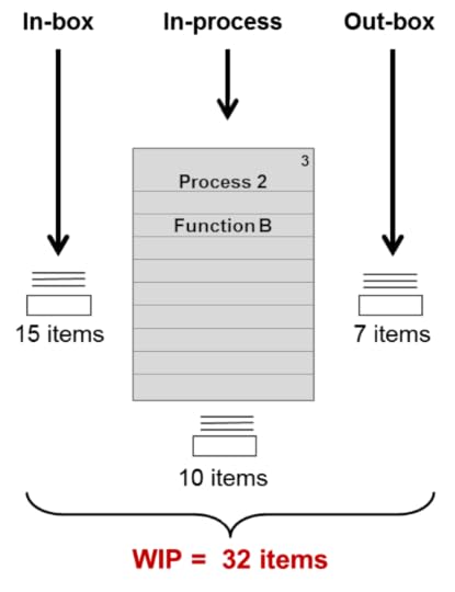
Note, too, that WIP can accumulate during any of the three stages bulleted above. We typically include WIP on our value stream maps to see where the largest queuing and constraints lie versus using those numbers to calculate the lead time. (However, in high volume office “production” areas with dedicated resources, the lead time will approximate WIP/daily demand).

As you can see on the sample value stream maps in our book’s Appendices and on the VSM segment shown later in the post, the WIP for a particular process is shown to the left of the process block and includes WIP from any of the three stages listed above:

Timeline Treatment

Sadly, there is no industry-wide standard for value stream metrics and timeline conventions. Some people break process time into value-adding and non-value-adding time and show the sum for each category. Some people separate pure waiting time from the lead time rather than viewing it as total throughput time. Some people use the traditional square-wave timeline shape (commonly referred to as “sawtooth” shape), while others use a straight line. And so on.

Until three years ago, I used the square-wave type timeline and placed the lead time on the “peak” of the timeline to the left of the process block it referred to. And I placed process time in the “trough” of the timeline directly below the process block it referred to.

But over the years, I found that teams consistently got tripped up with which metric went where. And the metrics placement didn’t make intuitive sense to many teams when they had to reverse the placement in their minds in order to calculate Activity Ratio. Activity Ratio (AR) is a summary metric we use to reflect the degree of flow, which we’ve described in Value Stream Mapping (p. 90), as well as our two earlier books, The Kaizen Event Planner and Metrics-Based Process Mapping: AR = (Sum of timeline process times/Sum of timeline lead times) x 100. In the formula, process time is on top. On a sawtooth timeline, it’s on the bottom.

For these reasons, I eventually moved to a single line timeline, with process time on the top and lead time on the bottom. In the below example, process time is above the line and expressed in minutes, and the lead time is below the line and expressed in hours:

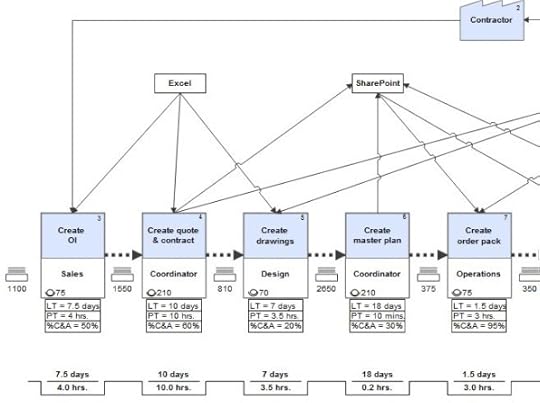
Unfortunately, our preferred software for creating electronic versions of maps (which aid in distribution and storage), iGrafx® FlowCharter, doesn’t yet have a straight line option for the timeline. But we found a workaround that enables us to place both metrics directly below the process block, which approximates a manually drawn straight line. However, due to iGrafx hard-coded conventions, the lead time remains on top. I share this because it answers the question we’ve gotten about why the timelines on the sample value stream maps we included in the Value Stream Mapping appendices look as they do:

So that’s the story. I hope this clarifies why and how we treat lead time the way that we do. I invite your comments and will continue to periodically post responses to the questions we’re getting, so please keep them coming.

As a reminder, I offer free monthly webinars where I cover topics such as this. You can learn about them by subscribing: www.ksmartin.com/subscribe.

You can also listen to the recordings for past webinars on our website, YouTube, Vimeo, and SlideShare (which also includes the slides). I’ve given six webinars on value stream mapping in the past six months, which you may find helpful.

Click here to register for my next value stream mapping webinar, hosted by Gemba Academy on Wednesday April 23 at 9 am Pacific Time.

And for more information on the book, visit www.ksmartin.com/value-stream-mapping. We give in-house value stream mapping workshops as well.

I wish you the best as you begin experimenting with or refine your use of value stream mapping to transform your value streams.