M.A. DeWitt's Blog

As part of a larger, ongoing project to develop decision-making and control algorithms for unmanned aerial vehicles, physics major, Spencer Ader, and I constructed a flight-data collection system. The goal was to be able to measure the throttle setting, control surface deflections, airspeed, angle of attack (angle between wing chord and oncoming airflow), and roll, pitch, and yaw angles in flight.

The first two sections of this post give a summary of the onboard computer, sensors, calibration functions, and sample data collected. The last three sections give details of how measurements are made, including the development of any models and empirical or semi-empirical relationships.

Contents




The Aircraft and SensorsFlight & Data SummaryMeasuring Control Surface Deflections & Static ThrustMeasuring AirspeedMeasuring Angle of Attack







The Aircraft and Sensors

(back to contents)

[image error] [image error] [image error] [image error] 707 false true true false true true false auto false ease-in-out 300 auto false 0 true false Previous (Left arrow key) Next (Right arrow key) %curr% of %total%

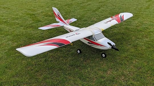
A radio-controlled E-flite Apprentice-S from Horizon Hobby was retrofit with a Raspberry Pi single board computer (SBC). In the fuselage, directly under the wing, is an open bay that holds the aircraft’s electronics. The Raspberry Pi and accompanying sensors were placed in this bay, mounted on a removable platform just above the aircraft’s control surface servos and electronic speed controller.

[image error] %curr% of %total%

The throttle setting of the aircraft was determined similarly. However, in this case, a force sensor was connected to the aircraft so that the force of static thrust could be measured for each PWM duty cycle. The data is summarized in the plot below of static thrust vs. tON. A linear fit to the data is also shown with the fit parameters. This thrust calibration function allows the static thrust to be calculated given the on time of the PWM signal.

Static thrust calibration curve. The points are data showing measurements of thrust force in Newtons at different PWM duty cycles. Rather than duty cycle, the on time of the PWM pulses are used here. A linear fit to the data is shown along with the fit parameters. Given the PWM time on, the static thrust developed by the motor and propeller can be calculated.







Measuring Airspeed

(back to contents)

In order to understand how airspeed can be measured, let’s first cover a couple of basic concepts. In everyday language, we speak of air as if it is either at rest or moving (e.g. wind). However, the molecules that make up the air around us (oxygen, nitrogen, etc) are in constant random motion, colliding with one another and with the objects they surround. We can think of these two types of motion—the small scale random motion of molecules and the orderly bulk motion of large numbers of molecules (i.e. wind)—as two distinct types of motion.

Pressure is usually thought of as a force distributed over an area. For example, at this very moment, molecules that make up the air surrounding your hand are colliding with it. The forces from the collisions result in a pressure. This is called static pressure because there is no bulk motion of the air and the collisions are due only to the small scale random motions of molecules. Since this happens all the time, we have become accustomed to this pressure and do not notice it. However, it is interesting to note that this pressure is almost 15 pounds of force per square inch! If we now impart some large-scale bulk motion to the air, say by using a fan, the air is no longer static. However, the random motions of the molecules do not cease. So, both motions are now present.  If you now place your palm in the stream of air coming from the fan, the molecules colliding with your hand will result in a pressure greater than the static pressure.  The amount of excess pressure, above static pressure, depends on the speed of the air stream. The greater the speed of the air, the greater the excess pressure is above the static pressure. If one could measure this excess pressure, one could work backward to determine the speed of the air. The measurement of this excess pressure is done using a pitot-static tube connected to a differential pressure sensor.

The internal chambers of a pitot-static tube.

A pitot-static tube (see above) contains two separate, concentric air chambers.  A hole in the front end of the tube is the opening of the first chamber, which runs along the length of the tube and through an exit port at the back of the tube. A piece of flexible tubing is used to connect this exit port to one side of a differential pressure sensor. Holes in the side of the pitot-static tube serve as the opening of the second chamber, which also runs along the length of the tube and through a second exit port. This port is connected to the other side of the differential pressure sensor, such that the differential pressure sensor measures the difference between the pressures in the two chambers of the pitot-static tube.

When the pitot-static tube is at rest, the pressure in each chamber is simply static pressure. Therefore, there is no pressure difference registered by the pressure sensor. If the pitot-static tube is placed in a moving stream of air, the air collides with the front face of the tube. At the opening, there is a point where the moving air is brought to a complete halt, called the stagnation point. Here, the total pressure (called stagnation pressure, Pstagnation) is the sum of the static pressure (Pstatic) and the excess pressure due to the bulk motion of the air. It turns out that this excess pressure (called dynamic pressure, Pdynamic) is proportional to the square of the speed of the air. Specifically, Pdynamic = ½ ρ V2, where ρ is the density of air, and V is its speed. This means that the pressure in the first chamber is the stagnation pressure

PChamber #1 = Pstagnation = Pstatic
Pdynamic = Pstatic  
½ ρ V2

Although the moving air collides with the front of the pitot-static tube, it flows smoothly over the sides of the tube. At the openings on the side, the bulk flow of air is not impeded like it is at the front of the tube. The airflow simply passes by the opening. Therefore, the only contributor to the pressure in the second chamber is the random motions of the molecules. This means that the pressure in this chamber is simply the static pressure

PChamber #2 = Pstatic.

Therefore, the differential pressure measured by the
pressure sensor is

ΔP = PChamber #1 – PChamber #2 = (Pstatic   ½ ρ V2) – Pstatic = ½ ρ V2,

which is just the dynamic pressure. Using this measurement of the dynamic pressure and knowing the density of air, the speed of the air can be calculated.

In order to calibrate the pitot-static tube and differential pressure sensor arrangement, we conducted measurements on the ground. The tube was attached to the side mirror of a car, and the tubing from the exit ports was run into the car through a cracked window. The differential pressure sensor was placed on the dashboard and connected to the I2C bus of a Raspberry Pi to collect the pressure measurements. The car was driven at a constant speed, while a digital anemometer was held out the passenger side window to measure the airspeed with significantly better precision than the car’s speedometer.

Using a system of rods and clamps, the Pitot-static tube was attached to the side mirror of a car. This setup was used to calibrate the pitot-static tube and differential pressure sensor on the ground before mounting it in the aircraft.



The differential pressure sensor and Raspberry Pi are mounted on the car’s dashboard. A lipo battery, stepped down through a UBEC powers the Pi and sensor. The Pi is connected to a laptop via an Ethernet cable and the Pi is accessed via SSH from a terminal.

A plot of the differential pressure versus airspeed is shown below. The blue dots are the data points taken using the differential pressure sensor and digital anemometer. As discussed above, the differential pressure, ΔP, should ideally be proportional to the square of the airspeed. The red line on the plot shows a quadratic fit to the data points, and the equation just below the legend gives the fit parameters.This is a calibration curve for airspeed, since it can be inverted to determine airspeed for a given differential pressure measurement.

Measuring Angle of Attack

(back to contents)

Angle of attack is defined as the angle between the oncoming airflow and the wing’s chord line. The chord line is an imaginary line connecting the leading and trailing edges of the wing cross-section.

The figure above shows the cross section of a wing. The front (or leading) edge is at the left of the figure, and the back (or trailing) edge is at the right. The imaginary line joining the leading and trailing edges is called the chord line. The angle between the chord line and the oncoming airflow is called the angle of attack, and is usually denoted with the Greek letter α. Angle of attack is an important quantity because the aerodynamic coefficients that characterize the lift, drag, and pitching moments for an aircraft are written as functions of α. The maximum angle of attack (known as the critical angle of attack) for most any wing is typically in the range of 15 – 20 degrees. If the angle of attack is increased beyond this critical value, instead of the air flowing smoothly over the wing, it tends to separate from the wing, dramatically decreasing the lift. This condition is known as a stall.

The measurement of the angle of attack is somewhat challenging. Manufacturers of modern airliners use a vane that sticks out of the fuselage into the airflow and is able to rotate to align with it. Measuring the angle of rotation of the vane gives the angle of attack.

Angle of attack vane. The vane rotates to align with the oncoming airflow.

We considered something similar; a rotating vane protruding from the side of the aircraft attached to an angular orientation sensor inside the fuselage. However, the presence of the propeller creates a somewhat turbulent wake near the aircraft and it was not clear how much this would affect the vane. We also wanted the measurement to be as simple as possible, avoiding any unnecessary moving parts. Since we had pitot-static tubes readily available, we decided to test how the differential pressure reading varied when the probe was held at different angles to the airflow. Perhaps this would serve as a useful way to measure angle of attack.

To collect some preliminary data, we attached two pitot-static tubes to the side mirror of a car; one of them pointing straight ahead and the other tilted downward at some angle.

The data we collected quickly revealed a problem. When the pitot-static tube is tilted, the air does not flow smoothly over the holes in the side of the tube. Some air rams into the hole that is angled toward the front. As the air flows around the tube, the other side holes each experience a different pressure. This caused erratic differential pressure readings for the tilted probe. To remedy this, the static port of the tilted probe was disconnected from the differential pressure sensor. A tee joint was used to tap into the static pressure line of the forward facing pitot-static tube, and connect it to the tilted probe’s differential pressure sensor. This way, both pressure sensors used the same, stable static pressure for comparison. Once this change was made, the following data was obtained. This is a plot of the differential pressure reading on the tilted probe (ΔP2) versus the differential pressure reading for the forward facing probe (ΔP1) for various tilt angles.

Recall from the section on measuring airspeed that the higher the airspeed, the higher the differential pressure reading for a forward facing pitot-static tube (ΔP). Therefore, the values of ΔP1 on the horizontal axis correspond to different airspeeds. Each set of data on the plot corresponds to a particular tilt angle for the second probe. These angles are specified in the legend. Note that for a fixed tilt angle, there appears to be a linear relationship between the pressure reading of the tilted probe (ΔP2) and the pressure reading of the forward facing probe (ΔP1). Linear fits to the data collected at each angle are shown on the plot. As the tilt angle increases, the slope of the linear relationship becomes less positive, passes through zero somewhere near 45 degrees, and then becomes negative.

In
order to use this information to determine angle of attack, for a given ΔP1 reading, the differential pressure readings for different angles of the tilted probe must be distinguishable. Recall that the critical angle of attack for most any wing is below 20 degrees. For the airfoil on our aircraft, it is somewhere near 15 degrees. On the plot, the data and fit lines for 0 degrees, 5 degrees, and 10 degrees practically lie on top of each other. So, it is not possible to distinguish a tilt of even 10 degrees. In terms of measuring angle of attack, this is bad news. However, for measuring airspeed, this is actually a good thing. This means that the pressure reading on a pitot-static tube that points forward is not very sensitive to relatively small changes in the angle of the airflow.
Therefore, for an angle of attack below 10 degrees or so, the airspeed
determined from the pressure reading is still extremely accurate. However, we are looking for a way to measure angle of attack, so let’s examine the rest of the data.

As the angle increases, the pressure reading ΔP2 becomes increasingly sensitive to small changes in the tilt angle. For example, take at the 46 degree and 56 degree lines. This is a spread of 10 degrees, and there is a significant difference between the values of ΔP2 at a fixed value of ΔP1. This means that if we were to mount a second pitot-static probe on the aircraft, such that it was tilted downward at a fixed angle of, say 50 degrees, then its differential pressure reading would be sensitive to small changes in the tilt angle. In other words, small upward or downward changes in the angle of attack would result in significant, measurable changes in ΔP2. Mounting the probe at a relatively steep angle would make its differential pressure reading useful for measuring angle of attack.

Before proceeding, there is another aspect of the data that is important to note. The values of ΔP2 display a significant spread about the fit lines. However, as the angle increases to 80 degrees and beyond, the spread in the measurements becomes considerably smaller. While the physical cause of this is unclear, it is sufficient to make note of the effect in order to minimize measurement error. The decision was made to mount a second pitot-static probe on the aircraft tilted downward at an angle of 80 degrees from the forward facing pitot-static probe. The pressure readings from this second probe would be sensitive to small changes in angle of attack, and the low measurement error would result in relatively small uncertainties in the predictions. The images below show how the two pitot-static tubes were mounted on the underside of the aircraft’s wing.

While
this gave a general method for measuring angle of attack, it remained to derive
a specific calibration curve that would allow the angle to be calculated in
terms of the pitot-static tube differential pressure readings. Consider what
happens at the front of the pitot-static tube as it is tilted away from the
forward position (see image below). When the tube is pointed forward, the
stagnation point, where the flow comes to a complete stop, is in the middle of
the opening in the tip. Because, the stagnation point is at the opening, the
differential pressure (total – static) measured by the sensor would be the
dynamic pressure ½ρV2 as discussed in the section on
measuring airspeed.

When the tube is tilted, the stagnation point is no longer at the opening. As the flow accelerates around the tip, the pressure at the surface drops below the stagnation pressure. Therefore, the total pressure at the opening of the pitot tube will be less than the stagnation pressure. This means that the differential pressure measured by the pressure sensor will be less than the full dynamic pressure. It is clear that this is the case from our earlier plot of ΔP2 vs. ΔP1 where, for a fixed value of ΔP1, as the tilt angle increases, the differential pressure ΔP2 decreases.

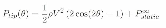
As a working model of the flow around the tip, we used the well-known case of the theoretical flow around an infinitely long cylinder (see image below). The red dots indicate stagnation points where the air is at rest. The speed, V, and static pressure are the values far from the cylinder (hence the use of infinity ∞).

The equation in the image above gives the total pressure on the surface of the cylinder at each point defined by the angle θ. For example, if θ = 0 degrees this refers to the stagnation point on the left side of the cylinder. This means we have cos(0 deg) = 1, and the equation reduces to Psurface = ½ ρV2 Pstatic,∞. This is just the stagnation pressure, as it should be. As another example, if θ = 30 degrees, we have cos(60 deg) = 1/2, and the equation reduces to Psurface = Pstatic,∞. This is less than the stagnation pressure. If we roughly model the flow around the pitot-static tube as the flow around a cylinder, we can use this equation to model the total pressure at the opening in the tip of the tube for different tilt angles. That is

Recall that the differential pressure sensor measures the difference between the total pressure at the tip and the static pressure. Therefore, the equation that describes the differential pressure sensor measurement can be derived as follows:

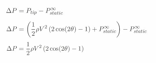
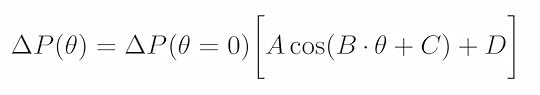
For a forward facing pitot-static tube, the angle between the tube and airflow is θ = 0 degrees, and the equation for the differential pressure measurement gives ΔP1 = ½ ρV2. For a pitot-static tube tilted at the angle θ, the differential pressure measurement is ΔP2 = ½ ρV2 [2cos(2θ) – 1]. Note that the factor of ½ ρV2 , which is the full dynamic pressure, is the differential pressure measured for zero tilt angle ΔP(θ = 0). Substituting ΔP(θ = 0) for the term ½ ρV2 allows us to write the differential pressure measured by a pitot-static tube as

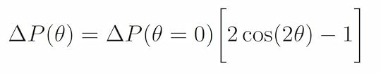
Recall that the earlier plot of ΔP2 vs. ΔP1 showed that ΔP2 was proportional to ΔP1 for a fixed tilt angle. The equation above reflects this fact, since ΔP1 = ΔP(θ = 0). Note that the proportionality constant is simply the function of theta in square brackets. On the earlier plot, this proportionality constant, for a particular tilt angle, would be the slope of the linear fit line. Using the slopes of the linear fits at different tilt angles, the following plot of slope vs. tilt angle was generated. Note that the symbol β is used for the tilt angle in this plot instead of θ.

For a number of reasons, including the fact that the tip of the pitot tube is not exactly cylindrical, we would not expect the data in the above graph to exactly follow the theoretical function [2cos(2θ) – 1]. However, using a more general cosine fit equation

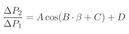
where A, B, C, and D are fit constants, we obtain the solid line through the data in the plot above. The fit parameters for this are:

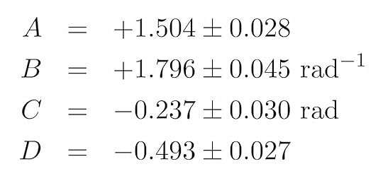
Given all the differences between the real pitot-static tube tip and an idealized cylinder, it is rather remarkable that this fits the data as well as it does. Note that the fit seems to be better at tilt angles above 0.6 rad (or about 34 degrees). Perhaps this has something to do with the size of the hole in the front of the pitot tube. Nonetheless, we have a calibrated relationship between the differential pressure measurement and the angle between the probe and the oncoming airflow.

How do we use this relationship to obtain the angle of attack? On the aircraft, there are two pitot-static tubes. One is mounted facing forward such that the tube is parallel with the wing chord. Therefore, the angle between the airflow and the forward facing tube is the same as the angle between the airflow and the wing chord, which by definition is the angle of attack (see image below). Note that the angle of attack is positive when the tube is tilted upward with respect to the airflow and negative when tilted downward. The second pitot-static tube is mounted so that it is tilted 80 degrees below the forward facing pitot-static tube. This means that the angle between the airflow and this second pitot-static tube is (80 deg – α).

Using
our fit equation to write the differential pressure measurements for each of
the pitot-static tubes, we obtain (note that 80 degrees is approximately 1.396
radians):

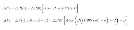
Taking the ratio of these two measurements (ΔP2 / ΔP1) yields

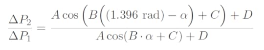
Therefore, if we measure the differential pressure for each pitot-static tube and then calculate the ratio of these measurements (ΔP2 / ΔP1), we can use above equation to numerically solve for the angle of attack, α.

The post Flight Data Collection System appeared first on Martin A. DeWitt.

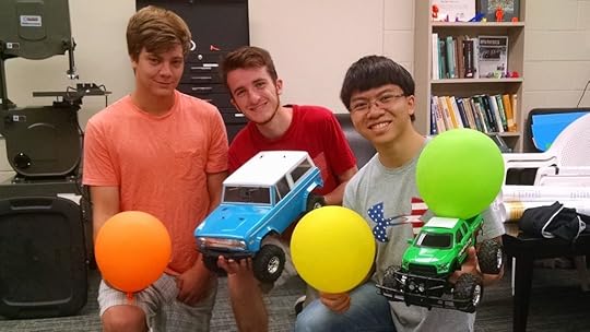Physics majors Max Maurer, Spencer Ader, and Ty Carlson (left to right).

In the summer of 2016, I worked with physics major Max Maurer, Spencer Ader, and Ty Carlson on a project that involved object detection, object tracking, and obstacle avoidance for a self-driving vehicle. The vehicle used was a 1/10th scale model of a 1972 Ford Bronco. We added a small USB camera and single-board computer (SBC) to the vehicle to serve as a vision system/brain. Both Raspberry Pi and ODROID XU4 SBCs were tested. The project was a mix of electronics, controls engineering, and image processing. All of the coding was done using Python, with extensive use of the Open Computer Vision (OpenCV) library.

The Vehicle and Electronics

Normally, a radio-controlled car is directly controlled by an onboard radio receiver, which is connected to a steering servo and an electronic speed controller (ESC). When the driver operates the controls on the handheld radio transmitter, the transmitter sends radio signals that are picked up by the receiver. The receiver interprets these signals and sends pulse-width modulated (PWM) signals via wires to control the steering servo and ESC. Since we wanted the vehicle drive itself, we bypassed the radio receiver, connecting the steering servo and ESC directly to an Adafruit PWM/Servo driver. The PWM/Servo driver was, in turn, wired to the onboard computer. This way, instructions could be sent from the computer to the driver, which would then send PWM signals to the steering servo and ESC.

The model Ford Bronco. Note the camera looking through the hole in the windshield.



Inside the Bronco. A Raspberry Pi and USB camera constitute the brain/vision system. In this first iteration, the PWM pins on the Raspberry Pi were connected directly to the steering servo and ESC. However, glitches with the PWM output necessitated using a PWM driver board which was added later.

The USB camera was connected directly to the onboard computer and was mounted to the inside roof of the Bronco, with the lens pointing through a hole cut in the windshield. Captured images were then processed using tools from the OpenCV library. The output of the image processing was used as input for making control decisions. A few different scenarios were investigated: having the vehicle (1) detect and track a known target (brightly colored balls or balloons), (2) follow a winding brick pathway, (3) detect and avoid known obstacles, and (4) avoid unknown obstacles.

A Brief Bit About Color Models

The information that is stored for a color digital image is simply a set of numbers that represent the intensity of red, green, and blue (RGB) light for each pixel. While RGB is the standard format, there is an alternative color model that stores numbers for Hue, Saturation, and Value (HSV). Hue is related to the wavelength of light in the visible spectrum. Saturation refers to the strength of the presence of a color as compared with pure white. Value refers to the lightness or darkness of a color. The HSV color model is often visualized using a cylinder (see below).

The HSV cylinder. (https://commons.wikimedia.org/wiki/User:Datumizer)

The HSV color model is more intuitively representative of the way humans perceive color. For example, imagine we take a picture of a yellow ball that is in full Sun, and then take another picture of the same ball in the shade under a tree. From the first to the second picture, the RGB numbers for each pixel would change in a way that is not necessarily intuitive. However, in the HSV model, the Hue would essentially remain the same, the Saturation may change slightly, and the Value would certainly become darker. This also tends to make HSV suitable for computer vision tasks that detect colored objects, especially in varying lighting conditions.

Detecting a Known Object Based on Color

Our first goal was to have the computer detect a yellow kickball. This was done using the back-projected histogram method. First, an image of the ball is used to construct a 2D histogram with binned values of Hue and Saturation for all of the pixels in the ball. For computational efficiency, the “Value” part of HSV was ignored. This Hue-Saturation (H-S) histogram was then used as a kind of filter for detecting the ball in other images.

An example of an image of the yellow ball and its H-S histogram is shown below. Because every pixel in the image of the ball has similar hues (around 50) and relatively similar saturation (from 150 – 250), the histogram is a sharp peak centered near a hue of 50 and saturation of 200.

Below is another example of an image and its corresponding H-S histogram. Note that this image has a wide variety of hue (greens, blues, etc) and saturation. Therefore, the H-S histogram shows structure at many different combinations of hue and saturation.

In order to determine whether the yellow ball is present in any given image, the image is analyzed pixel by pixel. For each pixel, the hue-saturation pair is compared with the yellow ball’s H-S histogram. The closeness of a given pixel’s hue-saturation pair to the peak in the yellow ball’s H-S histogram is used to generate a number that represents the probability that the pixel from the image is actually from the yellow ball. For example, if the H-S pair for a pixel in the image is (H, S) = (120, 40), this is far away from the yellow ball’s peak at (50, 200), so this pixel is assigned a very low probability of being the ball. However, if the H-S pair in the image is (48, 190), then it is much closer to the peak and is assigned a much higher probability of being the ball.

A probability value is generated for each pixel in the image. These probabilities are then used to construct a corresponding grayscale image known as a histogram back-projection. The back-projection has the same number of pixels (rows and columns) as the original image. Each pixel is assigned a grayscale value, with white being probability of 0 and black being a probability of 1. As an example, below is an image that contains the yellow ball. The grayscale image is the corresponding back-projection produced by the process described above. An algorithm can then be used to find the location of the ball by detecting the cluster of black pixels. Note that the white circle is not a ring of zero probability pixels, but rather a marker placed at the centroid of the black blob.

Tracking an Object of Interest

Once an object of interest can be isolated using a back-projection, OpenCV’s Continuously Adaptive MeanShift (CAMShift) algorithm can be used to track the object in real time. Recall that our object of interest shows up as a dark blob in a back-projection. In each successive video frame, the MeanShift algorithm uses a simple procedure to determine the magnitude and direction of the shift of the dark blob from its location in the previous frame. The continuously adaptive (CA) enhancement of the MeanShift algorithm keeps track of any change in size of the object, usually due to its changing distance from the camera. The information about the location and size of the object is then fed as input into a custom control algorithm to allow the vehicle to track a target at a fixed distance. This required the computer to steer the vehicle in order to keep the target in the center of the field of view, as well as to adjust the vehicle’s speed in order to maintain the following distance. Below is a test video of the vehicle tracking the yellow kickball.

Self-driving vehicle uses OpenCV’s CamShift algorithm and a custom
control algorithm to track a moving target.

We also attached a bright green balloon to the top of a second radio-controlled Ford Bronco to serve as a moving target. The video below is a first-person view from the camera onboard the self-driving vehicle.

First person view from the camera onboard the self-driving vehicle. The target is a green
balloon atop a second radio-controlled Ford Bronco. The blue square shows the location
and size of the object detected by OpenCV’s CamShift algorithm.








Follow the “Red” Brick Road!

With the ability to isolate and track an object of interest based on color, it was now a relatively simple matter to have the vehicle follow a winding pathway. The path we used was made of different shades of red brick. We stitched together a composite image of the various types of brick and used it to generate an H-S histogram. A histogram back-projection could then generated, showing the location of the brick path (see below). Note here that the grayscale colors are reversed; white pixels are a probability of 1 and black pixels are a probability of 0.

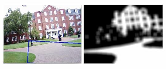
The geometric center of the brick material was then calculated, and the computer issued steering commands to keep this point in the center of the field of view. As you can tell from the above image, not only was the process successful at showing the brick path, but it showed the brick buildings as well. To remedy this problem, we had to mask off the top portion of the back-projection when computing the geometric center of the brick path. Below is a test video taken of the self-driving vehicle as it attempts to stay on the brick path.

Due to the vehicle’s short stature, the camera was very close to the ground making the brick fill up most of the bottom portion of the field of view. As a result of this loss of perspective cues, the vehicle was sometimes not able to tell if it was driving along the center of the path or at an angle toward the edge of the path. At times, the vehicle ended up driving at a right angle toward the edge of the path. In these cases, the edge of the path was a horizontal line across the field of view of the camera (see below).

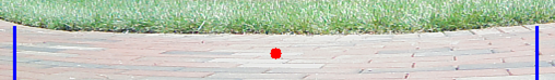Edge case: Heading straight for the edge of the path. Because the center of the brick path is in the center of the field of view, the vehicle continues to drive straight ahead, eventually running into the grass.

Unfortunately, this meant that the center of the brick path was in the middle of the image, so the vehicle just kept driving straight toward the edge of the path, eventually ending up in the grass. To solve this problem, we had the algorithm keep track of the percentage of the image that was brick. As the vehicle drove toward the edge of the path, more of this area would become filled with grass and the percentage of brick would shrink. At a certain threshold, the vehicle was programmed to begin slowing down and make a sharp turn in one direction to stay on the path.

Avoiding Known Obstacles

To incorporate obstacle avoidance into the self-driving vehicle’s capabilities, we took inspiration from the behavior of electrically charged particles. The characteristics of this behavior are well suited for developing a model of obstacle avoidance:

Like electrical charges (e.g. + and +) repel and unlike charges (+ and -) attract.The closer charges are to one another, the more strongly they attract or repel.The greater the magnitude of the charges, the more strongly they attract or repel.The overall (or net) force experienced by a single charge is a linear superposition of the forces caused by each of the charges surrounding it.

Using Item #1 in the list above, we think of the vehicle as having a positive electric charge. Targets are then considered to have a negative charge, while obstacles are considered to have a positive charge. As a specific example, consider the image below, which is taken from the self-driving vehicle’s camera and shows a single target (green balloon) and a group of obstacles (red, blue, and orange balloons).

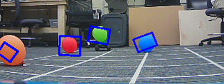First person view from the self-driving vehicle’s camera showing a target (green balloon) and three obstacles (orange, red, and blue balloons). The vehicle is a positive charge and the target is a negative charge. Therefore, the vehicle is attracted to the target. The obstacle balloons have a positive charge. Therefore, these balloons and the vehicle are repelled from one another.

For the target, the algorithm calculates a steering command that would tend to bring the target toward the center of the field of view (attract). Because the green balloon is close to the center of the image above, this would only require a small left turn. For an obstacle, the computer calculates a steering command that would cause the obstacle to move away from the center of the field of view (repel). Since the blue balloon is close to the center of the image, this would require a sharp turn to the left. The red balloon would require a slightly less sharp turn to the right. The orange balloon would require a fairly weak turn to the right. The specific steering commands are determined using graphs called steering curves. You can read about the steering curves in detail here if you are interested.

It is probably obvious that the vehicle can only receive one steering command to position the wheels. So, what happens when there are multiple objects like in the situation described above? This is where the principle of linear superposition (Item #4 on the list above) comes into play. For the sake of argument, let’s assign some arbitrary numerical values for the steering commands to see how this works. Let’s say a neutral steering command (no turn) is 0, a left turn command is a negative number, and a right turn command is a positive number. The sharper the turn required, the greater the magnitude of the command. So, for example, a very weak left turn might be -10, while a very strong right turn might be +100. In the image above, the green target would require a weak left turn to bring it to the center of the field of view. Using the letter ‘S’ to denote a steering command, let’s say this steering command is Sgreen = -10. Because it is close to the center, the blue obstacle requires a strong left turn to avoid. Let’s say Sblue = -80. The red balloon is a little farther away from the center, so perhaps the steering command to avoid it would be a moderate right turn of Sred = +60. Finally, the orange obstacle is close to the left edge, so it only requires a weak right turn of Sorange = +10 to avoid. In order to determine the net steering command to be sent to the servo, we take the superposition of these separate steering commands:

Snet = Sgreen + Sblue + Sred + Sorange = (-10) + (-80) + (+60) + (+10) = -20

So, the net steering command is -20. This is the command we actually send to the steering servo. This relatively weak left turn makes sense, as it sets a course between the red and blue obstacles, heading for the green target. Because the orange obstacle is so far to the left, this command will likely not bring us too close to it. In this way, the superposition helps the vehicle navigate its way through a field of obstacles.

Thus far, we have taken into account how close the object is to the center of the field of view when determining a steering command, however we have not yet considered the actual distance between the vehicle and object (Item #2 in the list above). Because we know the actual size of an object (i.e. balloon), we can use this along with its apparent size in the image to estimate the distance to it and use this information to place greater weight on the steering commands for nearby objects and less weight on the steering commands for far away objects. If we represent the weighting factor, w, as a function of distance, d, for object i as wi(di), then the distance weighted net steering command for n objects is:

Snet = w1(d1)*S1 + w2(d2)*S2 + . . . + wn(dn)*Sn

The net steering command is thus a weighted average of the individual steering commands for all of the objects in the vehicle’s field of view. Below are a some test videos that show the vehicle using this model to avoid obstacles and reach a target. The target is a green balloon attached to a small green RC vehicle.

Although we did not incorporate Item #3 from the list above, one could do so by imagining that different obstacles have different inherent levels of danger. For example, perhaps a red balloon is more dangerous than a blue balloon. Therefore, one could modify the weighting factors such that steering commands to avoid red balloons carry a greater weight than steering commands to avoid blue balloons.

Avoiding Unknown Obstacles Using Optical Flow

The final challenge was to have the vehicle avoid obstacles that were not known in advance. That is, we wanted the vehicle to be able to avoid any object placed in its path, not just brightly colored balloons. To accomplish this, optical flow was used to ???. Optical flow refers to the apparent movement of objects in a field of view due to the relative motion between the objects and the observer. This apparent motion could be due to the motion of the objects in the scene, the motion of the observer, or both. Consider the image below, which shows the view of a passenger looking out the window of a train. In the left frame the train is at rest, while in the right frame the train is moving to the right.

Because of parallax, objects closer to the train appear to move by faster (hence the blur), while distant objects appear to move by more slowly. If we place arrows on the objects in the scene to depict their apparent motion, with the arrowhead showing the direction and the length representing the speed, this would look something like the image below.

The red arrows visually depict the direction and speed of the apparent motion of objects in the passenger’s field of view. The collection of arrows is called an optical flow field.

One of OpenCV’s dense optical flow methods, which is based on Farneback’s algorithm , was used to produce optical flow fields for the scene viewed by the self-driving vehicle. An example is shown below. There are no arrowheads in this image, so note that the arrows begin at the blue dots and point along the red lines.

One shortcoming of using this method directly on images without any preprocessing (segmentation, etc) is that it is not possible for the routine to detect the motion of pixels in areas with little to no texture. In the image above, this is revealed in smooth areas like the large white patches of walls, ceiling, and floor. However, where there are distinct edges and texture — like around posters, doors, or even reflections of lights in the floor — the routine can detect the motion of pixels, hence the presence of optical flow vectors in these locations. In our tests, we used obstacles that had some level of surface texture to alleviate this issue.

How is the optical flow field useful in an obstacle avoidance framework? Objects that are farther away from the vehicle will have lower apparent speeds and therefore shorter optical flow vectors, while objects that are closer to the vehicle will have higher apparent speeds and therefore longer optical flow vectors. Rather than attempt to isolate individual objects, we simply divided the image in half with a vertical line. We then summed the lengths of the optical flow vectors on each side. Whichever side had the highest total was assumed to contain closer obstacles. Therefore, the vehicle was instructed to steer away from the side with the higher total.

The image below is from the point of view of the self-driving vehicle. The yellow numbers show the overall sums of the optical flow vector lengths for the left side (669) and right side (967) of the image. The large book in the foreground is contributing significantly to the higher total on the right. At this instant, the vehicle would be sent a steering command to turn to the left by an amount proportional to the difference between the total sums.

A test video of the vehicle using this obstacle avoidance method is shown below.

The post Self-driving Vehicle with Computer Vision appeared first on Martin A. DeWitt.

In the Spring of 2015, I and two first-year physics majors, Graham Rich and Max Maurer, participated in a high-altitude balloon project with the Python Piedmont Triad Users Group (PYPTUG). The project, led by PYPTUG organizer Francois Dion, and named “Team Near Space Circus” was supported by contributions from Inmar, Dion Research, and the High Point University Department of Physics.

The full payload consisted of 7 Raspberry Pi single-board computers (networked together), 7 Pi cameras, one PiNoir infrared camera, two sensor arrays to collect data, an APRS radio transmitter, a SPOT GPS tracker, and two 3s 4000mAh lipo batteries with UBECs to step the voltage down to 5 V so as to be compatible with the Raspberry Pis.  More details about the payload and the network can be found here on Francois Dion’s blog. All of these components were nestled inside of a hollow Styrofoam sphere with a diameter of about 40cm.

Graham, Max, and I assembled sensor arrays and wrote Python code to collect data from the sensors and store it on the Raspberry Pi’s SD card. The sensor arrays consisted of the BMP 180 Pressure Sensor, the HTU21D Humidity Sensor, and the LSM9DS0 9 degree-of-freedom Inertial Measurement Unit (IMU) from Sparkfun. The three sensors were soldered to a single PCB with their I2C buses connected together in parallel so that the array could be controlled with a single Raspberry Pi.  Two of these sensor arrays were created for redundancy.

The images below, show the payload components, including the two independent sensor arrays (yellowish PCBs with red Sparkfun sensor boards).

Bottom half of payload. Contains Raspberry Pi, cameras, and sensor arrays.



Top half of payload. Contains SPOT GPS tracker, APRS transmitter, and an upward facing camera.

Because the weather balloon bursts at some altitude, causing the payload to fall back to Earth, a parachute is attached just above the payload. Also, for safety, a radar reflector is attached just below the payload. The payload, parachute, and radar reflector were attached to a weather balloon with cord rated to break at a specific tension as dictated by the FAA. Rather than use a complicated system of gimbals to stabilize the payload, we instead used a system designed in 1912 by French engineer and WWI balloon pilot, Pierre Picavet.  The system is simply called a Picavet Suspension, and is commonly used in taking aerial photographs from kites.  For this project, the Picavet Suspension was made of a rigid cross of PVC pipe and monofilament fishing line looped through rings (see image below). As the cross tilts, the string slides through the loops allowing the payload to remain upright. You can see a video of the suspension in action and read more about it here.

Above the payload, a parachute is attached to control the descent of the balloon. For safety, a radar reflector is attached below the payload.

A close up of the Picavet suspension made from PVC pipe, plastic and metal rings, and monofilament fishing line.

The launch took place on April 21, 2015 from RayLen Vineyards in Mocksville, NC (just west of Winston-Salem) at 7:55am. Below are images showing preparations prior to the launch.

[image error] [image error] [image error] [image error] [image error] [image error] [image error] [image error] [image error] 548 false false true false true true false auto false ease-in-out 300 false 0 true false Previous (Left arrow key) Next (Right arrow key) %curr% of %total%

A video of the launch itself. . .

The launch from the perspective of the payload. Prepare to get dizzy!

As the balloon ascends, the atmospheric pressure outside the balloon decreases. This causes the balloon to expand until it eventually ruptures. The series of images below was taken from an upward facing camera and shows the balloon at various altitudes along its ascent. Note the change in size.

[image error] [image error] [image error] [image error] [image error] [image error] [image error] [image error] [image error] [image error] [image error] [image error] 327 false false true false true true false auto false ease-in-out 300 false 0 true false Previous (Left arrow key) Next (Right arrow key) %curr% of %total%

When the balloon finally ruptures, the payload slows to stop and then tumbles and falls. The series of images below were again taken from the upward facing camera and shows the balloon at various altitudes along its descent.  Unfortunately, we missed the exact moment of rupture, so the first image is just afterward.  The next couple of images show significant distortion of the Picavet cross, indicating abrupt rotation. Eventually, the parachute opens, stabilizing and slowing the descent.  In the final image, the payload has settled in a very short tree, which made recovery easier than anticipated. The parachute as well as the radar reflector (silver object near the top center of the final image) are easily identified.

[image error] [image error] [image error] [image error] [image error] [image error] [image error] [image error] [image error] 335 false false true false true true false auto false ease-in-out 300 false 0 true false Previous (Left arrow key) Next (Right arrow key) %curr% of %total%

The payload landed at 9:39am in Hurdle Mills, North Carolina, roughly 100 miles East Northeast of the launch site. An analysis of the pressure sensor data revealed that the maximum altitude reached by the balloon had been about 80,000 ft above sea level. Below are plots of the pressure sensor data, as well as plots of the altitude and ascent or descent rate derived from the pressure data. The stated operating range of the SparkFun BMP180 pressure sensor gives the lowest calibrated pressure as 30,000 Pa. This corresponds to an altitude of about 30,000 ft. above sea level. Therefore, it is not clear how accurate the pressure data was after the balloon passed 30,000 ft. The manufacturer of the weather balloon claims a burst altitude of between 95,000 ft and 105,000 ft, although this depends on the payload weight and level of inflation. Given this, together with the fact that the balloon continued to ascend for about 45 minutes after passing 30,000 ft makes it plausible that the maximum altitude could have been in the neighborhood of 80,000 ft or even higher.

[image error] [image error] [image error] [image error] 607 false false true false true true false auto false ease-in-out 300 false 0 true false Previous (Left arrow key) Next (Right arrow key) %curr% of %total%

The post High-Altitude Balloon appeared first on Martin A. DeWitt.

50 Shades of Grey changed the face of erotica forever. Books from the genre were previously hidden in the XXX back section of stores (if they had a section at all). Some writers felt strange writing it and readers felt dirty even picking the books up. Through the combination of accessibility and digital anonymity, people started reading these steamy books out in the open. They’re everywhere. A friend who works at an airport bookstore told me that erotica is all they sell now! Erotica has officially joined the mile high club.

I’ve always loved writing erotic scenes, but I never considered the challenge of writing erotica because it felt like there was too much of a stigma behind it. In addition, I like infusing my scenes with comedy. I didn’t think that sex and comedy went together in this genre, until a bunch of parody books trying to capitalize on the success of 50 Shades began to pop up.

They were funny and sexy.

That settled it. I was going to write a sexy and funny book, but I wanted to base it not on 50 Shades but on a classic tale that everybody would know. Romeo and Juliet almost immediately popped into my head. I’ve been a bit of a Shakespeare nut for years and the thought of revisiting his most popular work for the sake of erotic parody made me very excited. The bard is already funny and sexy, so my biggest challenge has been making the work my own. I think I’ve done that, but I’ll let all of you be the judge of whether or not I’ve been successful when it comes out at the end of October.

If the book is a hit, I’m not going to stop there. I’m going to make it a part of the Sensual Shakespeare Series. My challenge: adapt all 37 of Shakespeare’s plays into erotic parodies. Can I do it? Would people want me to do it? Sound off in the comments below or send me a message to let me know if you think it’s a good idea.

Thanks for visiting the site!

Sincerely,

M.A.