As part of a larger, ongoing project to develop decision-making and control algorithms for unmanned aerial vehicles, physics major, Spencer Ader, and I constructed a flight-data collection system. The goal was to be able to measure the throttle setting, control surface deflections, airspeed, angle of attack (angle between wing chord and oncoming airflow), and roll, pitch, and yaw angles in flight.

The first two sections of this post give a summary of the onboard computer, sensors, calibration functions, and sample data collected. The last three sections give details of how measurements are made, including the development of any models and empirical or semi-empirical relationships.

Contents




The Aircraft and SensorsFlight & Data SummaryMeasuring Control Surface Deflections & Static ThrustMeasuring AirspeedMeasuring Angle of Attack







The Aircraft and Sensors

(back to contents)

[image error] [image error] [image error] [image error] 707 false true true false true true false auto false ease-in-out 300 auto false 0 true false Previous (Left arrow key) Next (Right arrow key) %curr% of %total%

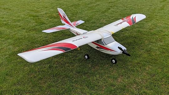
A radio-controlled E-flite Apprentice-S from Horizon Hobby was retrofit with a Raspberry Pi single board computer (SBC). In the fuselage, directly under the wing, is an open bay that holds the aircraft’s electronics. The Raspberry Pi and accompanying sensors were placed in this bay, mounted on a removable platform just above the aircraft’s control surface servos and electronic speed controller.

[image error] %curr% of %total%

The throttle setting of the aircraft was determined similarly. However, in this case, a force sensor was connected to the aircraft so that the force of static thrust could be measured for each PWM duty cycle. The data is summarized in the plot below of static thrust vs. tON. A linear fit to the data is also shown with the fit parameters. This thrust calibration function allows the static thrust to be calculated given the on time of the PWM signal.

Static thrust calibration curve. The points are data showing measurements of thrust force in Newtons at different PWM duty cycles. Rather than duty cycle, the on time of the PWM pulses are used here. A linear fit to the data is shown along with the fit parameters. Given the PWM time on, the static thrust developed by the motor and propeller can be calculated.







Measuring Airspeed

(back to contents)

In order to understand how airspeed can be measured, let’s first cover a couple of basic concepts. In everyday language, we speak of air as if it is either at rest or moving (e.g. wind). However, the molecules that make up the air around us (oxygen, nitrogen, etc) are in constant random motion, colliding with one another and with the objects they surround. We can think of these two types of motion—the small scale random motion of molecules and the orderly bulk motion of large numbers of molecules (i.e. wind)—as two distinct types of motion.

Pressure is usually thought of as a force distributed over an area. For example, at this very moment, molecules that make up the air surrounding your hand are colliding with it. The forces from the collisions result in a pressure. This is called static pressure because there is no bulk motion of the air and the collisions are due only to the small scale random motions of molecules. Since this happens all the time, we have become accustomed to this pressure and do not notice it. However, it is interesting to note that this pressure is almost 15 pounds of force per square inch! If we now impart some large-scale bulk motion to the air, say by using a fan, the air is no longer static. However, the random motions of the molecules do not cease. So, both motions are now present.  If you now place your palm in the stream of air coming from the fan, the molecules colliding with your hand will result in a pressure greater than the static pressure.  The amount of excess pressure, above static pressure, depends on the speed of the air stream. The greater the speed of the air, the greater the excess pressure is above the static pressure. If one could measure this excess pressure, one could work backward to determine the speed of the air. The measurement of this excess pressure is done using a pitot-static tube connected to a differential pressure sensor.

The internal chambers of a pitot-static tube.

A pitot-static tube (see above) contains two separate, concentric air chambers.  A hole in the front end of the tube is the opening of the first chamber, which runs along the length of the tube and through an exit port at the back of the tube. A piece of flexible tubing is used to connect this exit port to one side of a differential pressure sensor. Holes in the side of the pitot-static tube serve as the opening of the second chamber, which also runs along the length of the tube and through a second exit port. This port is connected to the other side of the differential pressure sensor, such that the differential pressure sensor measures the difference between the pressures in the two chambers of the pitot-static tube.

When the pitot-static tube is at rest, the pressure in each chamber is simply static pressure. Therefore, there is no pressure difference registered by the pressure sensor. If the pitot-static tube is placed in a moving stream of air, the air collides with the front face of the tube. At the opening, there is a point where the moving air is brought to a complete halt, called the stagnation point. Here, the total pressure (called stagnation pressure, Pstagnation) is the sum of the static pressure (Pstatic) and the excess pressure due to the bulk motion of the air. It turns out that this excess pressure (called dynamic pressure, Pdynamic) is proportional to the square of the speed of the air. Specifically, Pdynamic = ½ ρ V2, where ρ is the density of air, and V is its speed. This means that the pressure in the first chamber is the stagnation pressure

PChamber #1 = Pstagnation = Pstatic
Pdynamic = Pstatic  
½ ρ V2

Although the moving air collides with the front of the pitot-static tube, it flows smoothly over the sides of the tube. At the openings on the side, the bulk flow of air is not impeded like it is at the front of the tube. The airflow simply passes by the opening. Therefore, the only contributor to the pressure in the second chamber is the random motions of the molecules. This means that the pressure in this chamber is simply the static pressure

PChamber #2 = Pstatic.

Therefore, the differential pressure measured by the
pressure sensor is

ΔP = PChamber #1 – PChamber #2 = (Pstatic   ½ ρ V2) – Pstatic = ½ ρ V2,

which is just the dynamic pressure. Using this measurement of the dynamic pressure and knowing the density of air, the speed of the air can be calculated.

In order to calibrate the pitot-static tube and differential pressure sensor arrangement, we conducted measurements on the ground. The tube was attached to the side mirror of a car, and the tubing from the exit ports was run into the car through a cracked window. The differential pressure sensor was placed on the dashboard and connected to the I2C bus of a Raspberry Pi to collect the pressure measurements. The car was driven at a constant speed, while a digital anemometer was held out the passenger side window to measure the airspeed with significantly better precision than the car’s speedometer.

Using a system of rods and clamps, the Pitot-static tube was attached to the side mirror of a car. This setup was used to calibrate the pitot-static tube and differential pressure sensor on the ground before mounting it in the aircraft.



The differential pressure sensor and Raspberry Pi are mounted on the car’s dashboard. A lipo battery, stepped down through a UBEC powers the Pi and sensor. The Pi is connected to a laptop via an Ethernet cable and the Pi is accessed via SSH from a terminal.

A plot of the differential pressure versus airspeed is shown below. The blue dots are the data points taken using the differential pressure sensor and digital anemometer. As discussed above, the differential pressure, ΔP, should ideally be proportional to the square of the airspeed. The red line on the plot shows a quadratic fit to the data points, and the equation just below the legend gives the fit parameters.This is a calibration curve for airspeed, since it can be inverted to determine airspeed for a given differential pressure measurement.

Measuring Angle of Attack

(back to contents)

Angle of attack is defined as the angle between the oncoming airflow and the wing’s chord line. The chord line is an imaginary line connecting the leading and trailing edges of the wing cross-section.

The figure above shows the cross section of a wing. The front (or leading) edge is at the left of the figure, and the back (or trailing) edge is at the right. The imaginary line joining the leading and trailing edges is called the chord line. The angle between the chord line and the oncoming airflow is called the angle of attack, and is usually denoted with the Greek letter α. Angle of attack is an important quantity because the aerodynamic coefficients that characterize the lift, drag, and pitching moments for an aircraft are written as functions of α. The maximum angle of attack (known as the critical angle of attack) for most any wing is typically in the range of 15 – 20 degrees. If the angle of attack is increased beyond this critical value, instead of the air flowing smoothly over the wing, it tends to separate from the wing, dramatically decreasing the lift. This condition is known as a stall.

The measurement of the angle of attack is somewhat challenging. Manufacturers of modern airliners use a vane that sticks out of the fuselage into the airflow and is able to rotate to align with it. Measuring the angle of rotation of the vane gives the angle of attack.

Angle of attack vane. The vane rotates to align with the oncoming airflow.

We considered something similar; a rotating vane protruding from the side of the aircraft attached to an angular orientation sensor inside the fuselage. However, the presence of the propeller creates a somewhat turbulent wake near the aircraft and it was not clear how much this would affect the vane. We also wanted the measurement to be as simple as possible, avoiding any unnecessary moving parts. Since we had pitot-static tubes readily available, we decided to test how the differential pressure reading varied when the probe was held at different angles to the airflow. Perhaps this would serve as a useful way to measure angle of attack.

To collect some preliminary data, we attached two pitot-static tubes to the side mirror of a car; one of them pointing straight ahead and the other tilted downward at some angle.

The data we collected quickly revealed a problem. When the pitot-static tube is tilted, the air does not flow smoothly over the holes in the side of the tube. Some air rams into the hole that is angled toward the front. As the air flows around the tube, the other side holes each experience a different pressure. This caused erratic differential pressure readings for the tilted probe. To remedy this, the static port of the tilted probe was disconnected from the differential pressure sensor. A tee joint was used to tap into the static pressure line of the forward facing pitot-static tube, and connect it to the tilted probe’s differential pressure sensor. This way, both pressure sensors used the same, stable static pressure for comparison. Once this change was made, the following data was obtained. This is a plot of the differential pressure reading on the tilted probe (ΔP2) versus the differential pressure reading for the forward facing probe (ΔP1) for various tilt angles.

Recall from the section on measuring airspeed that the higher the airspeed, the higher the differential pressure reading for a forward facing pitot-static tube (ΔP). Therefore, the values of ΔP1 on the horizontal axis correspond to different airspeeds. Each set of data on the plot corresponds to a particular tilt angle for the second probe. These angles are specified in the legend. Note that for a fixed tilt angle, there appears to be a linear relationship between the pressure reading of the tilted probe (ΔP2) and the pressure reading of the forward facing probe (ΔP1). Linear fits to the data collected at each angle are shown on the plot. As the tilt angle increases, the slope of the linear relationship becomes less positive, passes through zero somewhere near 45 degrees, and then becomes negative.

In
order to use this information to determine angle of attack, for a given ΔP1 reading, the differential pressure readings for different angles of the tilted probe must be distinguishable. Recall that the critical angle of attack for most any wing is below 20 degrees. For the airfoil on our aircraft, it is somewhere near 15 degrees. On the plot, the data and fit lines for 0 degrees, 5 degrees, and 10 degrees practically lie on top of each other. So, it is not possible to distinguish a tilt of even 10 degrees. In terms of measuring angle of attack, this is bad news. However, for measuring airspeed, this is actually a good thing. This means that the pressure reading on a pitot-static tube that points forward is not very sensitive to relatively small changes in the angle of the airflow.
Therefore, for an angle of attack below 10 degrees or so, the airspeed
determined from the pressure reading is still extremely accurate. However, we are looking for a way to measure angle of attack, so let’s examine the rest of the data.

As the angle increases, the pressure reading ΔP2 becomes increasingly sensitive to small changes in the tilt angle. For example, take at the 46 degree and 56 degree lines. This is a spread of 10 degrees, and there is a significant difference between the values of ΔP2 at a fixed value of ΔP1. This means that if we were to mount a second pitot-static probe on the aircraft, such that it was tilted downward at a fixed angle of, say 50 degrees, then its differential pressure reading would be sensitive to small changes in the tilt angle. In other words, small upward or downward changes in the angle of attack would result in significant, measurable changes in ΔP2. Mounting the probe at a relatively steep angle would make its differential pressure reading useful for measuring angle of attack.

Before proceeding, there is another aspect of the data that is important to note. The values of ΔP2 display a significant spread about the fit lines. However, as the angle increases to 80 degrees and beyond, the spread in the measurements becomes considerably smaller. While the physical cause of this is unclear, it is sufficient to make note of the effect in order to minimize measurement error. The decision was made to mount a second pitot-static probe on the aircraft tilted downward at an angle of 80 degrees from the forward facing pitot-static probe. The pressure readings from this second probe would be sensitive to small changes in angle of attack, and the low measurement error would result in relatively small uncertainties in the predictions. The images below show how the two pitot-static tubes were mounted on the underside of the aircraft’s wing.

While
this gave a general method for measuring angle of attack, it remained to derive
a specific calibration curve that would allow the angle to be calculated in
terms of the pitot-static tube differential pressure readings. Consider what
happens at the front of the pitot-static tube as it is tilted away from the
forward position (see image below). When the tube is pointed forward, the
stagnation point, where the flow comes to a complete stop, is in the middle of
the opening in the tip. Because, the stagnation point is at the opening, the
differential pressure (total – static) measured by the sensor would be the
dynamic pressure ½ρV2 as discussed in the section on
measuring airspeed.

When the tube is tilted, the stagnation point is no longer at the opening. As the flow accelerates around the tip, the pressure at the surface drops below the stagnation pressure. Therefore, the total pressure at the opening of the pitot tube will be less than the stagnation pressure. This means that the differential pressure measured by the pressure sensor will be less than the full dynamic pressure. It is clear that this is the case from our earlier plot of ΔP2 vs. ΔP1 where, for a fixed value of ΔP1, as the tilt angle increases, the differential pressure ΔP2 decreases.

As a working model of the flow around the tip, we used the well-known case of the theoretical flow around an infinitely long cylinder (see image below). The red dots indicate stagnation points where the air is at rest. The speed, V, and static pressure are the values far from the cylinder (hence the use of infinity ∞).

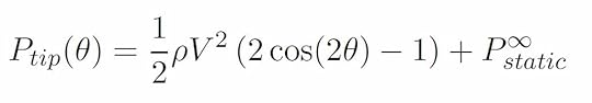
The equation in the image above gives the total pressure on the surface of the cylinder at each point defined by the angle θ. For example, if θ = 0 degrees this refers to the stagnation point on the left side of the cylinder. This means we have cos(0 deg) = 1, and the equation reduces to Psurface = ½ ρV2 Pstatic,∞. This is just the stagnation pressure, as it should be. As another example, if θ = 30 degrees, we have cos(60 deg) = 1/2, and the equation reduces to Psurface = Pstatic,∞. This is less than the stagnation pressure. If we roughly model the flow around the pitot-static tube as the flow around a cylinder, we can use this equation to model the total pressure at the opening in the tip of the tube for different tilt angles. That is

Recall that the differential pressure sensor measures the difference between the total pressure at the tip and the static pressure. Therefore, the equation that describes the differential pressure sensor measurement can be derived as follows:

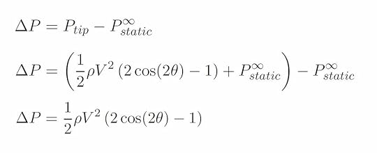
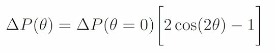
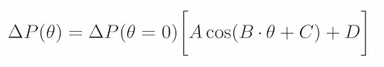
For a forward facing pitot-static tube, the angle between the tube and airflow is θ = 0 degrees, and the equation for the differential pressure measurement gives ΔP1 = ½ ρV2. For a pitot-static tube tilted at the angle θ, the differential pressure measurement is ΔP2 = ½ ρV2 [2cos(2θ) – 1]. Note that the factor of ½ ρV2 , which is the full dynamic pressure, is the differential pressure measured for zero tilt angle ΔP(θ = 0). Substituting ΔP(θ = 0) for the term ½ ρV2 allows us to write the differential pressure measured by a pitot-static tube as

Recall that the earlier plot of ΔP2 vs. ΔP1 showed that ΔP2 was proportional to ΔP1 for a fixed tilt angle. The equation above reflects this fact, since ΔP1 = ΔP(θ = 0). Note that the proportionality constant is simply the function of theta in square brackets. On the earlier plot, this proportionality constant, for a particular tilt angle, would be the slope of the linear fit line. Using the slopes of the linear fits at different tilt angles, the following plot of slope vs. tilt angle was generated. Note that the symbol β is used for the tilt angle in this plot instead of θ.

For a number of reasons, including the fact that the tip of the pitot tube is not exactly cylindrical, we would not expect the data in the above graph to exactly follow the theoretical function [2cos(2θ) – 1]. However, using a more general cosine fit equation

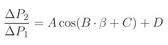
where A, B, C, and D are fit constants, we obtain the solid line through the data in the plot above. The fit parameters for this are:

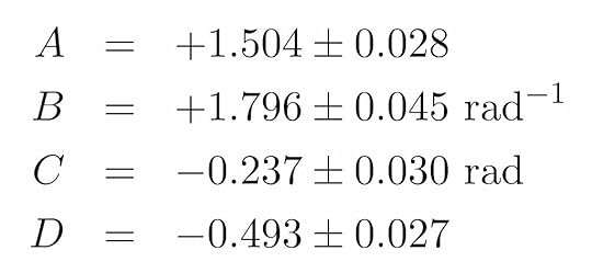
Given all the differences between the real pitot-static tube tip and an idealized cylinder, it is rather remarkable that this fits the data as well as it does. Note that the fit seems to be better at tilt angles above 0.6 rad (or about 34 degrees). Perhaps this has something to do with the size of the hole in the front of the pitot tube. Nonetheless, we have a calibrated relationship between the differential pressure measurement and the angle between the probe and the oncoming airflow.

How do we use this relationship to obtain the angle of attack? On the aircraft, there are two pitot-static tubes. One is mounted facing forward such that the tube is parallel with the wing chord. Therefore, the angle between the airflow and the forward facing tube is the same as the angle between the airflow and the wing chord, which by definition is the angle of attack (see image below). Note that the angle of attack is positive when the tube is tilted upward with respect to the airflow and negative when tilted downward. The second pitot-static tube is mounted so that it is tilted 80 degrees below the forward facing pitot-static tube. This means that the angle between the airflow and this second pitot-static tube is (80 deg – α).

Using
our fit equation to write the differential pressure measurements for each of
the pitot-static tubes, we obtain (note that 80 degrees is approximately 1.396
radians):

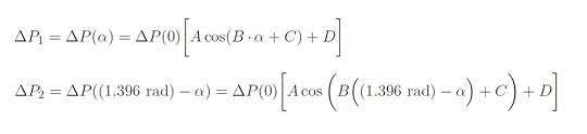
Taking the ratio of these two measurements (ΔP2 / ΔP1) yields

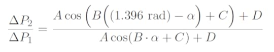
Therefore, if we measure the differential pressure for each pitot-static tube and then calculate the ratio of these measurements (ΔP2 / ΔP1), we can use above equation to numerically solve for the angle of attack, α.

The post Flight Data Collection System appeared first on Martin A. DeWitt.