One of my ongoing research interests is understanding the nature of technological progress: How does new technology come into the world and improve over time? What sort of factors affect it? How, in general, should we think about it? I’ve come at this question from a few different angles: posts looking at the operations and legacy of Bell Labs, posts looking at how specific technologies improved over time, posts looking at how frequent multiple invention is and how long we wait for new inventions, and so on.

My current line of thinking is that creating some new technology is best thought of as a search process. A given technology can be thought of as a point in some high-dimensional “design space” or “technology space,” which contains every possible technology: every conceivable arrangement of parts, materials, natural phenomena, and so on. The job of the would-be inventor is to navigate this space, sifting through the arrangements of elements that don’t work to find the ones that will.

This search process is made difficult by the fact that, as with any situation where you’re enumerating the possible combinations of a large number of elements, technology space is incomprehensibly vast. In “Are Technologies Inevitable?” economist Matt Clancy notes that Wikipedia listed 272 “named equations” that describe various regularities in the world, ranging from the Navier-Stokes equations (which describe the motion of fluids) to the Arrhenius equation (which describes chemical reaction rates as a function of temperature) to the Exner equation (which describes how sediment gets deposited in a river). If we use this as a (very rough) estimate as to the number of different phenomena that a technology can leverage, it implies an enormous number of possible technologies that could be created. As Clancy writes:

If we’ve got 272 regularities to work with, for example, then the number of possible combinations of these regularities is two, raised to the power of 272 (since every regularity can be used or not used: two options). But 2^272 is more than some estimates of the number of atoms in the observable universe. And that’s got to be an undercount of the number of possible technologies, since it counts all technologies that use the same principles together as the same thing, even if they orchestrate them in vastly different ways or use them in vastly different magnitudes.

By comparison, the most common estimate for the number of atoms in the universe is around 10^80, or ~2^265. And it’s likely there are many, many more regularities that some technology could harness than 272. (Some in-progress work on this that I haven’t yet completed suggests that there are at least thousands.)

And as Clancy notes, this outrageously huge number dramatically undercounts the number of possible technologies, because it doesn’t take into account that the same phenomena can be used in lots of different ways. In Brian Arthur and Wolfgang Polak’s paper “The Evolution of Technology within a Simple Computer Model” (which we looked at earlier this year), Arthur and Polak note that even within the universe of logic circuits made up of three basic elements (the NAND gate and the values of 1 and 0), the number of different circuits you can make for even a small number of inputs and outputs is staggeringly large:

The emergence of circuits such as 8-bit adders seems not difficult. But consider the combinatorics. If a component has n inputs and m outputs there are (2^m)^(2^n) possible phenotypes, each of which could be realized in a practical way by a large number of different circuits. For example, an 8-bit adder is one of over 10^177,554 phenotypes with 16 inputs and 9 outputs.

So the search space for some new technology is vast. And the way that we tackle vast search spaces is with information. Each bit of information cuts a search space in half, so even a relatively small amount of information can quickly narrow down what seems like a huge search space. When we create some new technology, what we’re doing is gathering information: figuring out what will work and what won’t work, what’s promising and what isn’t, narrowing down the huge space of technological possibilities and finding something within it that accomplishes some particular goal.

In the 19th century, for instance, many people were interested in building a mechanical flying machine, but it wasn’t clear the exact arrangement of elements that would yield a successful one. Thanks to knowledge of the laws of physics, and an existence proof of birds, would-be inventors were already working within a considerably narrowed search space: they knew roughly what elements a flying machine would need to have — lifting surfaces, a propulsion system, and a means of control — and had a general idea of how they should be arranged. But there were a huge number of ways that you could build a flying machine from these basic elements, and people spent a great deal of time and effort building different sorts of machines that did not in fact work. The Wright brothers’ eventual success can in large part be attributed to the fact that they were exceptionally talented at gathering information, enabling them to converge on a working airplane design far faster than their competitors.

I previously explored the nature of technological search in that previous piece looking at Arthur and Polak technological evolution paper, which uses a simple simulation to evolve different logic circuits, finding workable technologies amidst an enormous sea of possibilities. I really liked the basic simulation method Arthur used in this paper — randomly generating technologies to see how easy or hard it was to find working ones — and wanted to use simulation myself to further explore the dynamics of technological search. But while Arthur uses digital circuits — different arrangements of logic gates like NAND, OR, AND, etc. that can perform functions like addition — I wanted a more general model that could capture the nature of many different types of technology, while still being simple enough to simulate easily.

The PTOP model

The model I came up with is inspired by another of Brian Arthur’s examinations of the nature of technology: his book The Nature of Technology. In this book Arthur describes technology as fundamentally “a set of phenomena captured and put to use.” He writes that:

… a practical technology consists of many phenomena working together. A radio receiver is not just a collection of parts. Nor is it merely a miniature signal processing factory. It is the orchestration of a collection of phenomena — induction, electron attraction and repulsion, electron emission, voltage drop across resistance, frequency resonance — all convened and set up to work in concert for a specific purpose.

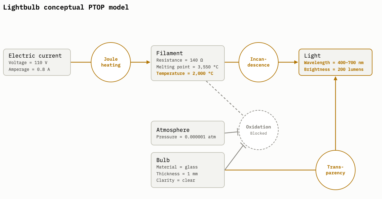
Edison’s lightbulb, for instance, took advantage of several different phenomena: Joule heating, the phenomenon that electric current running through a material will raise its temperature. Incandescence, the phenomenon that a hot enough object will emit light. Transparency, the phenomenon that certain materials will allow the passage of light. And so on.

Phenomena like this are typically triggered automatically when the right conditions are created, which you can think about as being when the right objects, with the right properties, are placed in some particular arrangement. In the lightbulb, Joule heating occurs automatically when electric current runs through the filament, and incandescence occurs automatically when the filament gets hot enough. And the bulb had a vacuum atmosphere to prevent another, unwanted phenomenon — carbon reacting with oxygen — automatically occurring and destroying the carbon filament.

These three elements — Phenomena, Objects, and Properties — are the basic components of the technological model I came up with, which I call PTOP, for Phenomena Triggered by Objects with Properties. In this model you have some collection of objects, which can have some specified set of properties. Whenever the right objects with the right properties are placed in the proper arrangement, a phenomenon will be automatically triggered, which can have various effects: modifying the properties of existing objects, creating new objects, and so on. By chaining the correct objects and phenomena together in the correct order, you can create your desired outcome, which is some particular object or objects with some specific set of desirable properties. A simple, conceptual PTOP model for the lightbulb, for instance, might look like this:

Via Opus 5.5.

By arranging the right sort of filament, an atmosphere, a bulb container, and electric current, you can trigger a series of phenomena that will ultimately result in the creation of light with desirable properties.

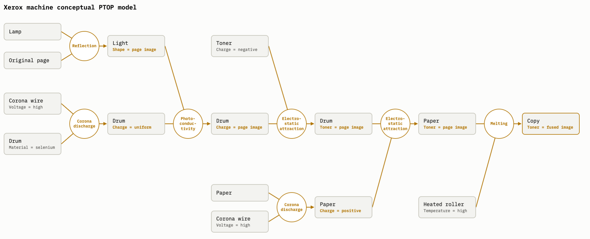
And here’s a sketch of a PTOP model for a more complicated technology, a Xerox machine, which uses various phenomena such as “photoconductivity” and “corona discharge” to generate a copy of a document:

Via Opus 5.5.

I like this model because it captures the basic elements — natural phenomena and the conditions that trigger them — inherent to all types of technology, such that we can study the ‘space’ of possible technologies. And you can implement the basic idea in many different ways, from very simple representations of technology to very complex ones. In some ways this is bad (it took me a super long time, for instance, to come up with a simulable implementation that I was happy with) but it’s useful for studying different aspects of technological search. Let’s look at a few different implementations of a PTOP model and see what we find.

A level 1 PTOP model

Let’s start with an extremely simple version of PTOP. In this version, we have 10 possible objects, each with two possible properties. The first property, P0, can take on any value from 1 to 10 and is inherent and unique to that object. You can think of this as the model having 10 different chemical elements, each taking on a different value of P0. The second property is size, which can also take on any value from 1 to 10, but is adjustable. So you can have a large object with P0 equal to 1 and size equal to 10, or a small object with P0 equal to 1 and size equal to 1. Overall there are 100 possible sorts of objects: 10 different object types, each of which can be 10 different sizes.

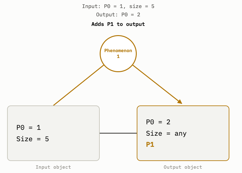
This version of the model has four phenomena in total. Each phenomenon is triggered when the right two objects are connected, and the first of those objects (what we’ll call the input object) has the correct size. When the phenomenon is triggered, it adds a specific property to the second object (what we’ll call the output object). So in the image below, when an object with a P0 value of 1 and size 5 is connected to an object with a P0 value of 2, it triggers a phenomenon, which adds a new property, P1, to the second object.

Via Opus 5.5.

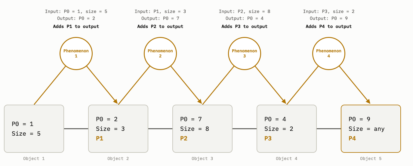
The phenomena in this model are arranged in a hierarchy: triggering each phenomenon requires an object with the property added by the previous phenomenon. So to trigger the phenomenon that adds P2, you need an object with the P1 property. P3, in turn, requires an object with P2, and so on. You can think of this hierarchy of phenomena as representing something like “to trigger incandescence, I need an object with a high temperature. To achieve high temperature, I need to use the phenomenon of Joule heating, which I can trigger with the right sort of electric current. To create electric current, I need …” and so on.

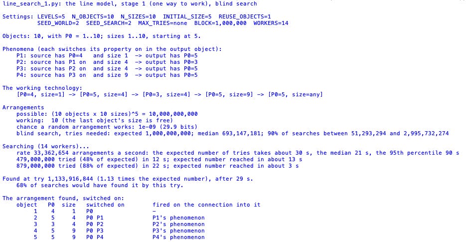
In this version of the model, the goal is to create an object with the “final” property of P4. You can think of this as representing something like “light with the proper brightness” or “lead shot with the proper size and sphericity.” This can be done by creating the exact right arrangement of objects: five objects arranged in a line, each with the correct P0 property and size.

Via Opus 5.5.

This is a very simple implementation of PTOP, which we’ll call a “level 1 model.” But it does capture a few things about the technological search process. First, the search space in even this very simple model is very large: 10 object types, 10 sizes, and 5 objects total means (10x10)^5 = 10 billion possible arrangements to produce a P5-level phenomenon.1 If you increased that to 100 objects, 100 sizes, and 10 different phenomena, you’d have 10^40 possible options. If we added more property types (maybe objects can have the properties of “temperature” and “density” in addition to size) the numbers would quickly become beyond astronomical.

But this simple version also shows the power that information can bring to bear on a large search space. When we looked at Arthur’s circuit search, we noted that what made the search tractable was modularity — finding a working design for a subcomponent, then locking that modular design into the system and using it as a repeatable ‘primitive’ element for further combinations. By preventing you from having to get every single part of a design correct in one shot, modularity effectively screens off many possibilities and reduces the size of the search space that must be traversed. As we found in that simulation:

A useful way of thinking about our 68 NAND gate search is that it’s like a huge, branching tree. At every step — every time we add a gate — there are thousands of branches, each one representing one possible way to wire up the gate. Each branch then splits into thousands more (representing all the possible ways of wiring up the next gate), which split into thousands more, which split into thousands more, until at the end we have 2^852 possible “leaves,” each one representing a unique way of wiring up all 68 gates. Trying to get all 68 gates right at once, and then checking to see whether or not you did, is like examining one single leaf, one path from the base of the tree all the way to the tip of a branch. Not only are you overwhelmingly likely to guess wrong, but you haven’t narrowed down your possibilities at all: all you know is that one single leaf wasn’t the right answer, leaving you with the rest of the 2^852 possible leaves to sift through.

Checking to see whether each gate we add is correct before we proceed to the next one, by contrast, massively narrows down the number of possibilities. Whenever we determine a gate isn’t in the right spot, it eliminates every possibility that branches off from that point. If there are 1000 possible ways to wire each gate, each time we guess correctly we’ve narrowed down the possibilities downstream of that choicepoint by 99.9%. Huge swaths of possibilities get eliminated at each correct guess, letting us converge on the correct answer much more quickly.

We can see these same basic mechanics with the PTOP model. With 10 object types, 10 sizes, 4 phenomena, and 1 billion effective possibilities, it takes (on average) 1 billion attempts to guess the entire correct design in one shot by randomly generating possible technologies.

But if we do a modular search — randomly adding just one object while randomly adjusting the size of the previous object until we’ve triggered the next phenomenon, then locking that successful design in and moving on — the search becomes much faster, because we’ve replaced a single billion-possibility space with a series of 100-possibility spaces. It takes on average 1,300 attempts to find the 10 type, 10 size, 4 phenomena answer, and even astronomically enormous technology space search problems become tractable.

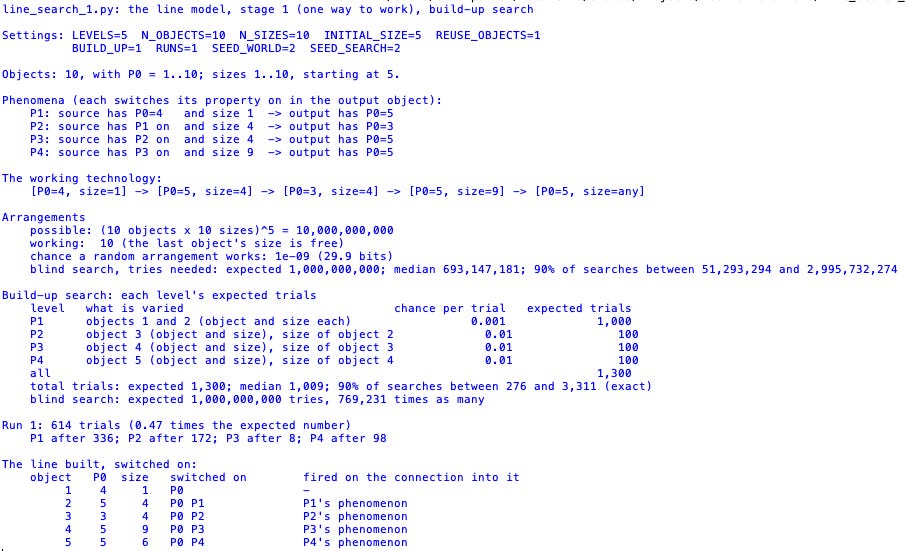
This version also shows that the degree of modularity makes a huge difference in how easy a technology is to find. The more modules we have whose design we can lock in, the shorter each step is up the ladder to the working technology, and the easier each step is to take. If we take our 10 object type, 10 size model up to 100 phenomena levels, we’re now at an enormous 10^200 search space, but with 100 steps up the ladder that we can lock in, finding it is trivial — a random search finds it after about 10,000 attempts on average. The same-sized search space generated from 10 phenomena levels but 10 billion possible object types and sizes (which only gives us 10 steps up the ladder, rather than 100) becomes utterly impossible to find randomly, even with modular search.

This version of the model also lets us see how different sorts of knowledge can make the search process easier. For instance, as Joel Mokyr notes in The Gifts of Athena, scientific knowledge is very useful when trying to create some new technology, because “the range of experimentation possibilities that needs to be searched over is far larger if the searcher knows nothing about the natural principles at work.” In our level 1 PTOP model, scientific knowledge would be something like “phenomenon 3 can’t work with object type 2” or “phenomenon 4 must have its two objects of equal size.”

The usefulness of this sort of scientific knowledge is a function of how many possibilities it screens off. The more possibilities it screens off, the more bits of information it provides, and the more useful it is. So something like “phenomenon 5 can’t use object 1” or “object 3 can’t touch object 4” provides a relatively small amount of information, because it doesn’t eliminate that many possibilities. Knowledge of the sort “phenomenon 4 MUST use object 1” or “object 3 MUST touch object 4,” by contrast, screens off a lot more possibilities, provides much more information, and narrows the search much more effectively.

!function(){"use strict";window.addEventListener("message",(function(e){if(void 0!==e.data["datawrapper-height"]){var t=document.querySelectorAll("iframe");for(var a in e.data["datawrapper-height"])for(var r=0;r<t.length;r++){if(t[r].contentWindow===e.source)t[r].style.height=e.data["datawrapper-height"][a]+"px"}}}))}();

One reason that, in the real world, the technological development process is tractable is that a lot of our knowledge is of the latter type. Phenomena typically have specific triggering conditions, which we can observe and discover: Marconi knew what was needed to create electromagnetic waves when he was working on his radio, Edison knew what was needed to create incandescence in a lamp filament, and the scientists on the Manhattan Project knew roughly what conditions were needed to trigger a nuclear chain reaction.

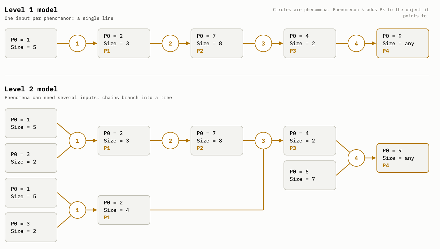
A level 2 PTOP model

Even this highly simplified version of the PTOP model is useful for exploring various technological search dynamics. But ultimately it’s a little too simple to capture many of the more interesting dynamics of technological search. So let’s add some complexity. First, real phenomena often require multiple “input” objects, rather than just one: triggering the phenomenon of “combustion” in a gasoline engine requires fuel, an oxidizer, and an electric spark. So we’ll make it so that each phenomenon can have multiple input objects instead of just one. Second, there are often multiple different phenomena that you can use to accomplish some particular goal: if you want to make mechanical motion, for instance, there are a variety of different phenomena you can harness to do that, and motors built to harness them — electric motors, hydraulic motors, internal combustion engines — all work in different ways. So let’s also make it so that instead of just one phenomenon for each level, there can be more than one, each one requiring a different set of objects with the right properties to trigger.

With the level 1 PTOP model, there was only a single workable version of the technology. With the level 2 model, there are multiple working designs. And unlike the straight lines of objects of the previous model, this one creates branching, treelike chains.

Via Opus 5.5.

With this version of the model (which I’ll call the “level 2 model”), even though there are a large number of possible working designs, the number of nonworking technologies is vastly larger, and finding a workable option by pure blind search quickly becomes unworkable.

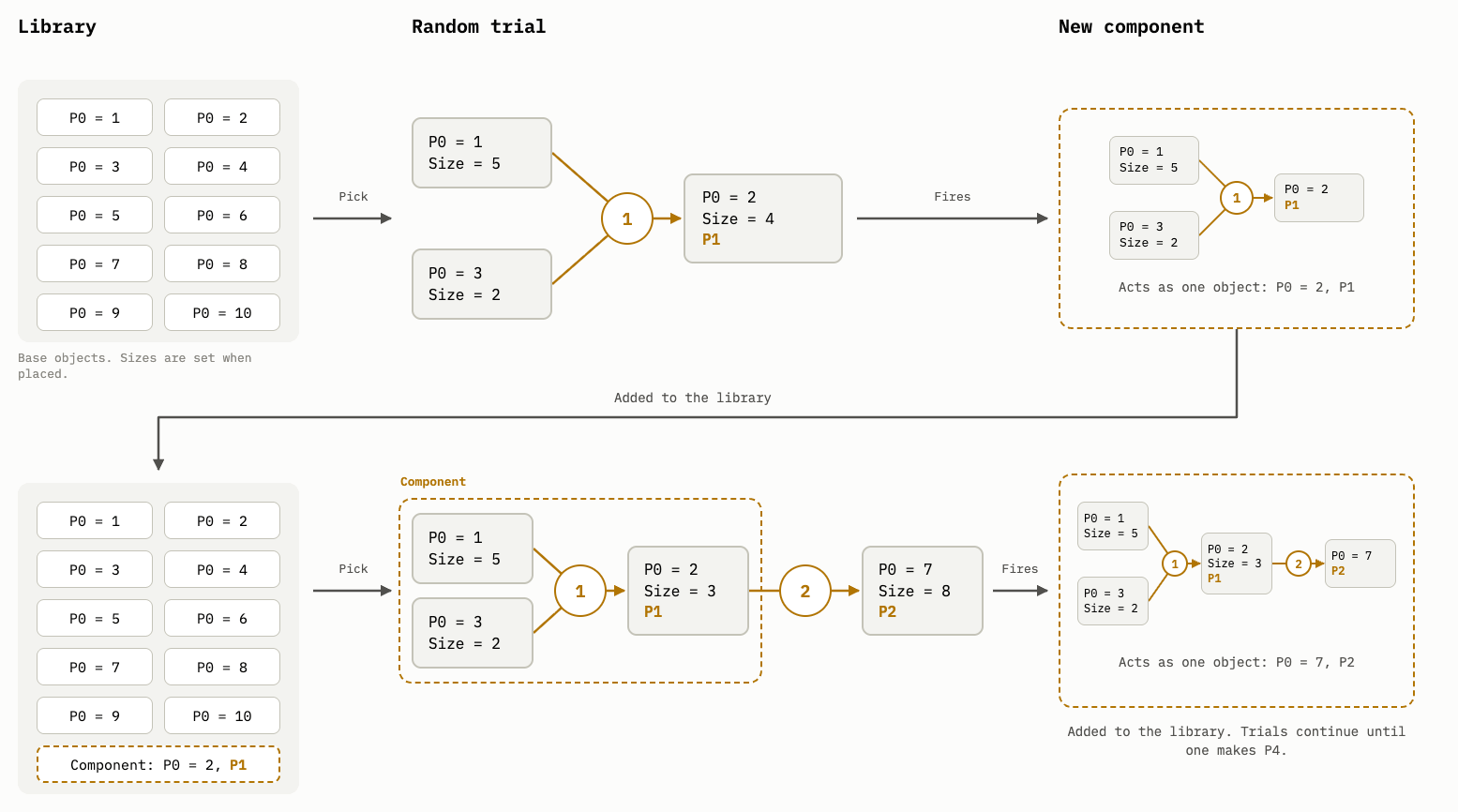
We can solve this with a slightly different flavor of modular search, very similar to the “encapsulation” that Arthur uses in his technological evolution paper. In this version, the model starts out by randomly combining different objects with different properties, connected in different ways. Whenever an arrangement of objects triggers some phenomena, that arrangement gets bundled into a new object, and then that object can be chosen by the simulation to be randomly combined with other objects. As with our previous, simpler modular search, this lets the simulation accumulate partial solutions and quickly find working technologies even amidst very large search spaces.

Via Opus 5.5.!function(){"use strict";window.addEventListener("message",(function(e){if(void 0!==e.data["datawrapper-height"]){var t=document.querySelectorAll("iframe");for(var a in e.data["datawrapper-height"])for(var r=0;r<t.length;r++){if(t[r].contentWindow===e.source)t[r].style.height=e.data["datawrapper-height"][a]+"px"}}}))}();

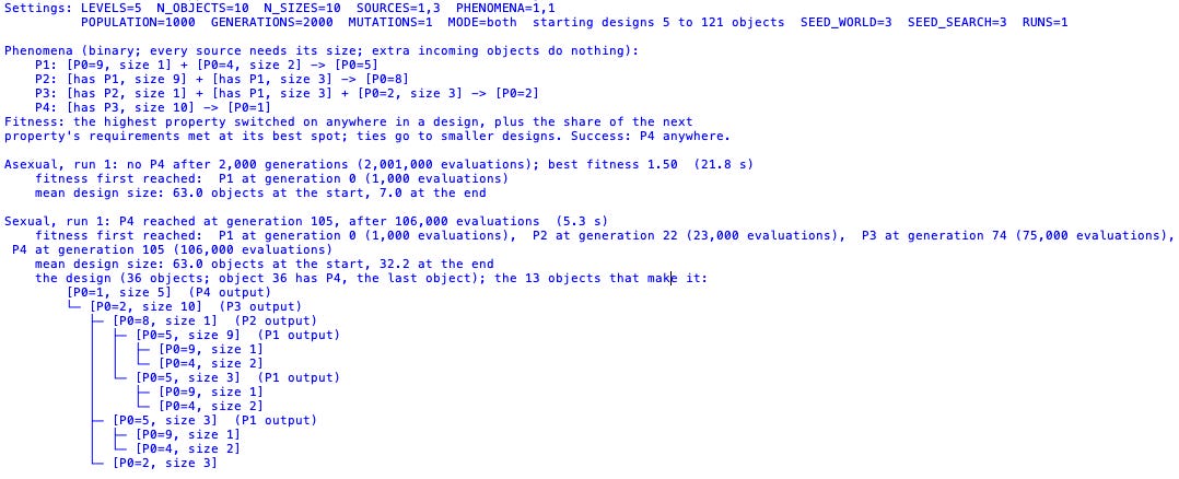
A level 2 PTOP model can also be used to show the information-accumulating power of sexual reproduction. In a previous essay, we noted that sexual reproduction is its own sort of modular search — by letting children inherit genes from two parents, sex allows useful genetic “discoveries” made by many different lineages to spread throughout the population. This is in contrast to asexual reproduction, where only one particular lineage ultimately survives, and discoveries made by others die out due to a phenomenon called “clonal interference.” This allows sexually reproducing populations to converge on maximum fitness much more quickly.

We can see this same thing using the level 2 PTOP model. I ran a version of it with two different technology “populations.” Each population had 1,000 randomly generated technologies in it. In one population, I implemented asexual reproduction — each generation, every technology would get one random mutation to an object (deleting an object, adding an object, or changing an objects properties). The fittest members of the population, measured by the highest phenomena level they had unlocked, survived into the next generation. In the other population, I implemented sexual reproduction — in addition to random mutation, children would be generated by randomly crossing over the branches of two parents. With 5 levels of phenomena, asexual reproduction couldn’t achieve the maximum phenomena level after 2,000 generations in the example below; sexual reproduction, by contrast, found it after just over 100 generations.

A level 3 PTOP model

This flavor of PTOP is a little richer and can show a broader array of technological search dynamics, but it’s still a little simple, so let’s add some more complexity.

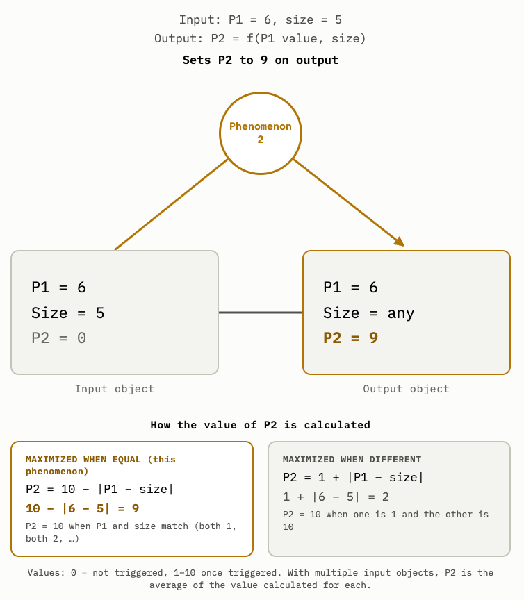
First, instead of making triggered properties — P1, P2, P3, etc. — binary (on or off), let’s make them be able to take on multiple values: before the property is switched on, it has a value of 0, while once a phenomenon triggers it, it can have a value from 1 to 10. We’ll make the value that it takes a function of two things: the size of the input object(s) and the value of the predecessor phenomenon. So for a phenomenon that triggers P2, the value of P2 will depend on the value of P1 and the size of its object. You can think of this as representing something like “the temperature in the lightbulb filament depends on the properties of the electric current flowing through it”: more amperage, or higher voltage, means higher filament temperatures. The brightness of the light emitted, in turn, will be a function of the temperature value of the filament.

We’ll make the value of triggered phenomena be determined in one of two ways. Either it’s maximized when the predecessor phenomenon and object size are EQUAL, or maximized when they’re as different as possible. So P2 can either be 10 when P1 and its size are the same (both 1, both 2, both 3), or when one is 10 and the other is 1. (For phenomena triggered by multiple input objects, we’ll take the average of the value calculated for each object.) We’ll call this version of the PTOP model the “level 3 model.”

Via Opus 5.5.

This change actually makes the initial stage of the technological search much easier. Because the correct object size is no longer needed to trigger a phenomenon (just the correct object type), getting a technology that triggers the final phenomenon is now very easy (though it would be easy to change this by making the value of triggered phenomena dependent on some new property instead of size, and keeping whether or not a phenomenon is triggered size dependent). But now there’s an element of performance tuning. A technology that works, in the sense that it has a positive value for the final triggered phenomenon, might be quick to find, but to maximize performance — achieve a final phenomenon with a value of 10 — you need to keep iterating, fiddling with the sizes of the various objects to gradually push performance up.

This dialing-in step is meant to capture the technological development process: taking some technology that already works to some degree and pushing its performance higher or building a version that works in a particular way. With Edison’s lightbulb, for instance, incandescent bulbs had been demonstrated since the early 19th century, but their performance was poor — they burned out quickly, or the interior of the bulb blackened, or they used too much power. Edison took a technology whose configuration had been mostly figured out — a high-melting-point filament, a glass bulb, and an atmosphere to minimize reactivity were all common characteristics of previous bulbs — and pushed its performance higher by tweaking the properties of the various elements: the level of vacuum, the size of the filament, the exact type of carbon, and so on.

In the level 2 model, we had multiple phenomena for each level — multiple different ways to trigger P2, for instance. In the level 3 model, we’ll keep the same feature, but we’ll add a twist: different phenomena have different ranges for triggered properties that they can possibly achieve. So one way of triggering P2 might only be able to reach a value of 7, while the other might be able to achieve a value of 10. For some technologies, this might be fine; in other cases, maximizing performance will require using some other, different phenomena instead.

This also mirrors what we see with real-world technologies. When developing some new technology, the designer will be confronted with many possible ways of doing some particular job, and depending on the performance required, different options might work best. In the lightbulb, the performance of a carbon filament could only be pushed so high, and so eventually lightbulbs switched to tungsten filaments, which in turn required inventing a new process for producing ductile tungsten wire. Similarly, there are a variety of different ways of implementing the valves on an internal combustion engine to let gases into and out of the cylinders. Achieving very high engine performance, such as the number of revolutions per minute required on a Formula One car, requires complex valves that use things like compressed air instead of conventional wire springs, while if you’re building a four-door sedan the cheaper and simpler wire spring is fine.

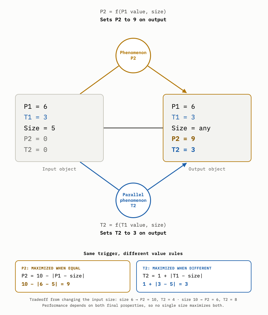
Let’s now add one more element to the level 3 model. Up until now, we’ve had one single chain of properties: one phenomenon triggers another, which triggers another, and so on. Now let’s add a parallel set of properties, triggered by a parallel set of phenomena. In our lightbulb example, we can think of this as the temperature of the filament triggering not only incandescence but thermal expansion and thermionic emission.

(In this example, all these phenomena are triggered by the same property, temperature. In our model, for ease of modeling purposes we’ll have each of the parallel phenomena triggered by its own property.)

These parallel phenomena are triggered under the same conditions as the primary phenomena, but their values might not necessarily be determined in the same way: the conditions that create a value of 10 for P2 might create a value of 5, or 1, for parallel property T2. Ultimate performance of a technology will be a function of both of the final triggered properties: the value of, say, not just P9 but T9 as well.

Via Opus 5.5

This addition has a few consequences. For one, the technological search becomes more difficult: trying to dial in a technology by adjusting sizes randomly takes many more iterations if you’re trying to maximize both P9 and T9 than it does if you’re just trying to maximize one or the other. This mirrors technology more generally: the more dimensions of performance you care about, the more difficult getting a technology that’s good enough is.

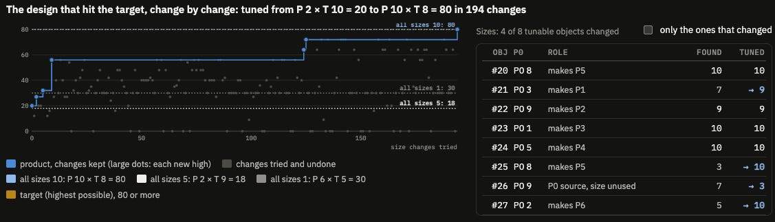Screenshot from one run of a level 3 model. For a given design, performance gradually improves as various size parameters are dialed in.

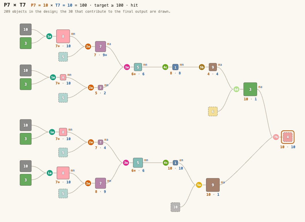
Another consequence of this addition is that we now have design trade-offs. With multiple phenomena (and parallel phenomena) at each level, we can have different designs, which might achieve different levels of performance. I ran a level 3 search that generated random technological prototypes, and then tried to dial in the performance of each one for several different performance goals: maximizing P7 and T7, minimizing them, and achieving some specific value for each. At the end of the run, each goal had a fundamentally different arrangement, with different values for object sizes. The same basic technology was best implemented in different ways, depending on the performance goal.

Screenshot from the same level 3 run as above. The combined goal (maximizing P7 x T7) took many more iterations to hit than either P7 alone or T7 alone. 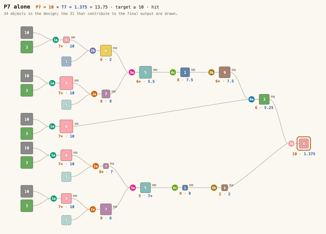Screenshots from a different level 3 run. The design that maximizes one value (P7) is different than the design that maximizes two values (P7 and T7). Conclusion

To understand the nature of technological progress, it’s useful to think of creating a new technology as a sort of search process, one that’s made tractable by the intelligent acquisition and application of information. We can understand technological progress, in turn, by studying the nature of search processes — what sort of things make them easy, what sort of things make them hard, what sort of information acquisition methods we can bring to bear, and so on. The PTOP models described above are, I think, a useful tool for exploring these technological search dynamics: they’re simple to simulate, they’re flexible, and they can capture a lot of real-world elements of technological development.

1

The actual search space is 1 billion, not 10, because the size of the last object doesn’t affect any phenomena.